Constraints and Profiles
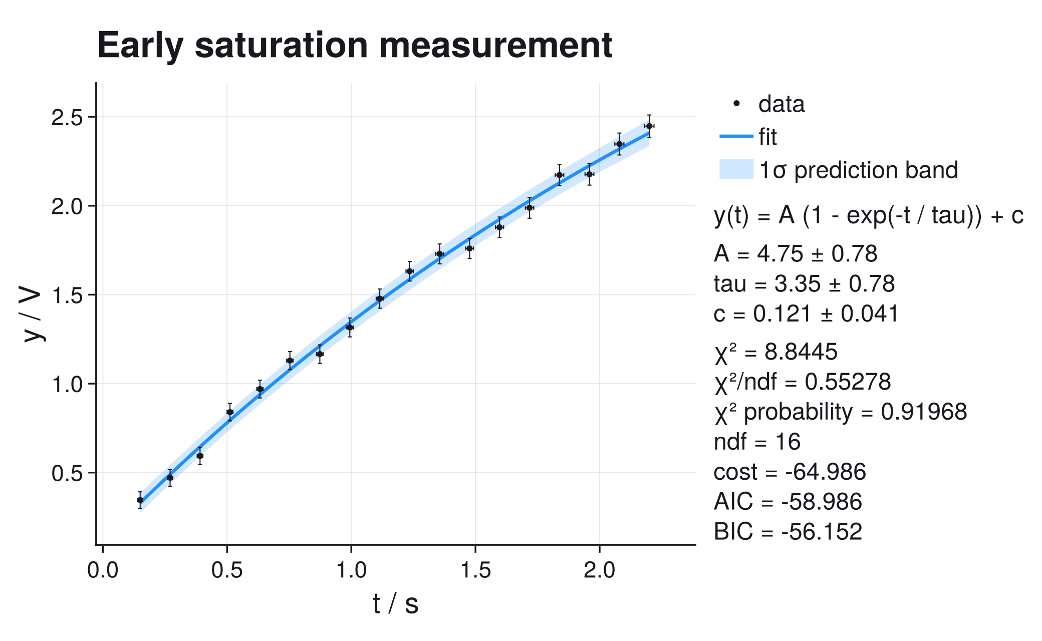
This workflow shows a case where the symmetric $\pm\sigma$ parameter errors taken from the local covariance matrix (param_stderr) are not enough: the fitted curve looks well determined over the measured interval, but two physical parameters remain strongly and nonlinearly coupled.
Scientific Question
A sensor approaches a steady response after a step input. Its expected response is
\[y(t) = A\left(1-e^{-t/\tau}\right) + c,\]
where $A$ is the response above baseline, $\tau$ is the time constant, and $c$ is the baseline. The measurement stops before the response reaches its plateau.
The analysis must answer:
- Can the available time window determine $A$ and $\tau$ separately?
- Is a symmetric covariance error a defensible uncertainty statement?
- How much does an independent baseline calibration help?
- What measurement should be added if the parameters remain degenerate?
Data
The controlled dataset below mimics an early-time step-response measurement: the plateau is not reached, each time point has its own uncertainty, and an independent baseline calibration supplies external information. It is a teaching record, not a measurement of a particular sensor. All four input arrays are printed in the fit cell; no hidden random generator or unknown true parameter enters the analysis.
The dataset includes individual absolute uncertainties in both time and response:
\[\sigma_{t,i} = 0.010 + 0.004t_i\ \mathrm{s}, \qquad \sigma_{y,i} = 0.045 + 0.008t_i\ \mathrm{V}.\]
An independent zero measurement supplies the Gaussian prior
\[c = 0.10 \pm 0.08\ \mathrm{V}.\]
Why The Parameters Become Degenerate
For times much shorter than the time constant,
\[1-e^{-t/\tau} \approx \frac{t}{\tau},\]
so the measured response is approximately
\[y(t) \approx \frac{A}{\tau}t + c.\]
Early data determine the ratio $A/\tau$ much better than $A$ or $\tau$ individually: a larger amplitude can be compensated by a longer time constant.
Bounds, Prior, And Cost
Amplitude and time constant must be positive. The fit enforces this through generous windows and keeps the baseline in a wide, physically plausible range:
\[0.1\ \mathrm{V} \le A \le 20\ \mathrm{V}, \qquad 0.1\ \mathrm{s} \le \tau \le 20\ \mathrm{s}, \qquad -0.5\ \mathrm{V} \le c \le 1.0\ \mathrm{V}.\]
The windows are deliberately loose: they exclude the unphysical branch without constraining the minimum.
The baseline calibration is uncertain external information, so it enters as a Gaussian term rather than a fixed value. Write the model as $f(t,p)$ with parameter vector $p=(A,\tau,c)$, so $f(t,p)=A\left(1-e^{-t/\tau}\right)+c$ is the response model from above. The effective variance of point $i$ is
\[s_i^2(p) = \sigma_{y,i}^2 + \left(\frac{\partial f(t_i,p)}{\partial t}\sigma_{t,i}\right)^2.\]
Because this effective variance depends on the fitted parameters, the default cost=:auto selects the full Gaussian likelihood cost on the $-2\log L$ scale; the fit cell below therefore passes no cost keyword:
\[C(p) = \sum_i \left[ \log\!\left(2\pi s_i^2(p)\right) + \frac{\left[y_i-f(t_i,p)\right]^2}{s_i^2(p)} \right] + \log\!\left(2\pi\,0.08^2\right) + \left(\frac{c-0.10}{0.08}\right)^2.\]
The sum is the Gaussian data term with the parameter-dependent effective variance; the last two terms are the $-2\log L$ contribution of the baseline prior, evaluated at the baseline component $c$ of $p$. In the fit cell below, model(t, p) implements $f$ with $A$ as p[1], $\tau$ as p[2], and $c$ as p[3].
The effective-variance approximation, its first-order validity range, and the role of the log-variance term are derived in Uncertainty In X.
Complete Fit
using CairoMakie
using ScientificFitting
using Printf

t = [
    0.150000, 0.270588, 0.391176, 0.511765, 0.632353, 0.752941,
    0.873529, 0.994118, 1.114706, 1.235294, 1.355882, 1.476471,
    1.597059, 1.717647, 1.838235, 1.958824, 2.079412, 2.200000,
]
response = [
    0.345641, 0.470693, 0.593535, 0.839840, 0.969673, 1.129630,
    1.165946, 1.315719, 1.477930, 1.631653, 1.729280, 1.759687,
    1.878716, 1.988480, 2.172411, 2.176549, 2.346881, 2.447489,
]
sigma_t = [
    0.010600, 0.011082, 0.011565, 0.012047, 0.012529, 0.013012,
    0.013494, 0.013976, 0.014459, 0.014941, 0.015424, 0.015906,
    0.016388, 0.016871, 0.017353, 0.017835, 0.018318, 0.018800,
]
sigma_response = [
    0.046200, 0.047165, 0.048129, 0.049094, 0.050059, 0.051024,
    0.051988, 0.052953, 0.053918, 0.054882, 0.055847, 0.056812,
    0.057776, 0.058741, 0.059706, 0.060671, 0.061635, 0.062600,
]

model(t, p) = @. p[1] * (1 - exp(-t / p[2])) + p[3]

result = fit_model(
    model,
    t,
    response;
    p0=[4.5, 3.0, 0.1],
    sigma_y=sigma_response,
    sigma_x=sigma_t,
    bounds=([0.1, 0.1, -0.5], [20.0, 20.0, 1.0]),
    parameter_priors=(index=3, mean=0.10, sigma=0.08),
    initial_guesses=[ # explicit starts are always tried in addition to p0
        [6.0, 5.0, 0.1],
        [3.0, 2.0, 0.1],
    ],
    maxiters=2000,
)

amplitude_interval = profile_interval(result, 1; npoints=81, nsigma=4)
amplitude_profile = amplitude_interval.profile_result
amplitude_timescale = ScientificFitting.contour(
    result,
    1,
    2;
    npoints=121,
    nsigma=4,
)
profile_overview = profile_matrix(
    result;
    parameters=[1, 2, 3],
    parameter_names=["A", "tau", "c"],
    npoints_profile=41,
    npoints_contour=21,
    nsigma=3,
    adaptive=true,
    max_refinements=1,
)

plot_profile(
    amplitude_profile;
    local_sigma=result.param_stderr[1],
    xlabel="amplitude A",
    title="Profile cost versus local parabola",
    delta_max=8,
)
plot_contour(
    amplitude_timescale;
    local_covariance=result.param_covariance,
    local_center=result.params[[1, 2]],
    xlabel="amplitude A",
    ylabel="time constant tau",
    title="Profile versus local covariance",
)
plot_profile_matrix(profile_overview)

@printf("amplitude = %.3f -%.3f +%.3f V\n",
        result.params[1],
        amplitude_interval.uncertainty_minus,
        amplitude_interval.uncertainty_plus)
@printf("profile interval = [%.3f, %.3f] V\n",
        amplitude_interval.lower,
        amplitude_interval.upper)
@printf("corr(A, tau) = %.4f\n", result.param_correlation[1, 2])
println(diagnostic_dashboard_text(result))amplitude = 4.750 -0.629 +1.018 V profile interval = [4.121, 5.768] V corr(A, tau) = 0.9928 Fit diagnostic dashboard status = review - inspect diagnostics critical = 0, warning = 2, info = 0 2 warning(s). Inspect before trusting uncertainties or conclusions. Next actions: 1. Use profile or contour intervals before treating symmetric covariance errors as final uncertainties. 2. Inspect a contour/profile plot. Re-center or rescale the independent variable, reparameterize the model, or add data that breaks the degeneracy.
Multiple starting points do not cure an under-informative experiment, but they make it less likely that a local optimizer accident is mistaken for the physical minimum.
The fit returns approximately (read from the result panel in the figure at the top of this page; programmatically result.params and result.param_stderr)
\[A = 4.75 \pm 0.78\ \mathrm{V}, \qquad \tau = 3.35 \pm 0.78\ \mathrm{s}, \qquad c = 0.121 \pm 0.041\ \mathrm{V}.\]
The near-equal errors on $A$ and $\tau$ are a coincidence of this dataset, not a typo. Those symmetric errors are only the local covariance summary; the fitted correlation between $A$ and $\tau$ of approximately $0.9928$ is already a warning to inspect the cost away from the minimum.
Diagnostics: Profile and Contour Checks
The profiles and contours answer whether the local covariance matrix is a faithful uncertainty summary or only a tangent approximation near the minimum.
Profile: Is The One-Parameter Error Symmetric?
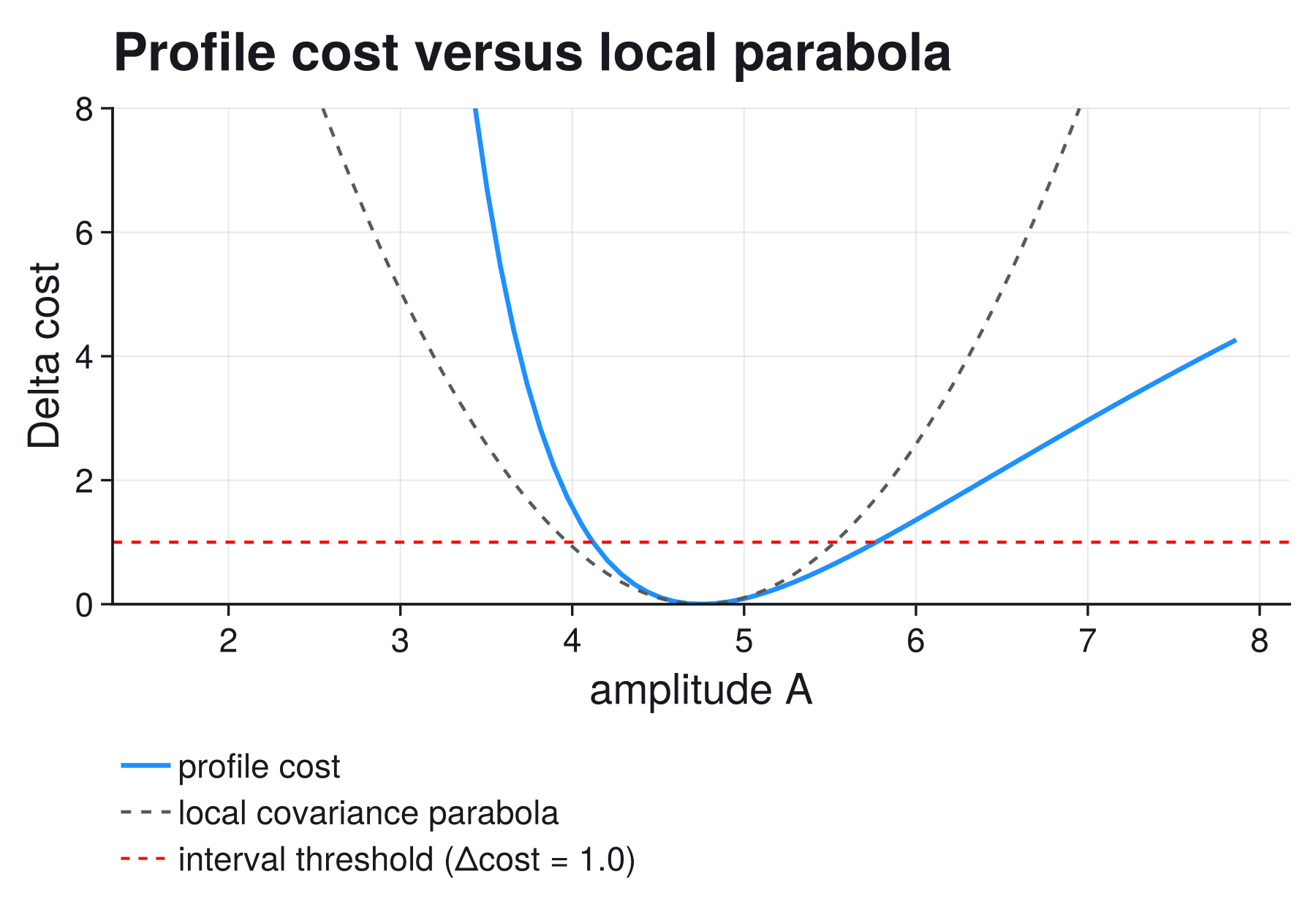
For every fixed amplitude, the profile scan refits $\tau$ and $c$ and records
\[\Delta C(A) = C\!\left(A,\widehat{\widehat{\tau}}(A), \widehat{\widehat{c}}(A)\right) - C_{\min}.\]
The double hat means "refitted while $A$ is held fixed," and $C_{\min}$ is the cost at the unconstrained best fit. The dashed parabola is what the local covariance matrix predicts:
\[\Delta C_{\mathrm{local}}(A) = \left(\frac{A-\hat A}{\sigma_A}\right)^2.\]
Here $\hat A = 4.75\ \mathrm{V}$ is the best-fit amplitude and $\sigma_A = 0.78\ \mathrm{V}$ its symmetric covariance error from above (result.param_stderr[1], passed to plot_profile as local_sigma).
The actual profile rises more slowly toward larger amplitudes. The one-sigma profile interval is approximately
\[A = 4.75^{+1.02}_{-0.63}\ \mathrm{V},\]
not $4.75 \pm 0.78\ \mathrm{V}$. The asymmetry is scientifically relevant: large amplitudes remain plausible because a longer time constant can hide the plateau beyond the measured interval.
The $\Delta C=1$ threshold and the assumptions behind it are derived in Profiles And Contours; the threshold line turns the scan into an interval construction rather than a qualitative curve inspection.
Contour: Which Parameter Combinations Survive?
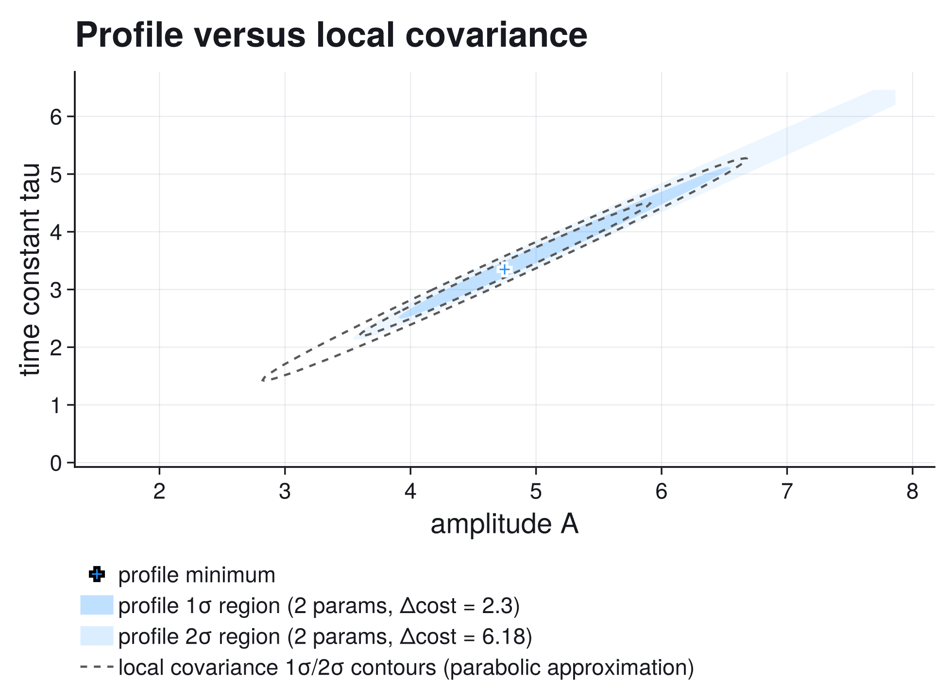
The filled regions are the actual profiled one- and two-sigma regions. At every grid point in $(A,\tau)$, ScientificFitting refits the baseline. The dashed curves are the local covariance ellipses.
For two parameters the thresholds are
\[\Delta C = 2.30 \quad \text{and} \quad \Delta C = 6.18\]
for one and two sigma respectively; why joint regions need different thresholds is explained in Profiles And Contours.
The profile region bends along combinations with similar early-time slope; the local ellipse cannot follow that curvature. Reporting only the covariance matrix would hide which high-$A$, high-$\tau$ combinations remain compatible with the measurement.
Matrix: Where Should You Look First?
For three or more fitted parameters, separate profile and contour plots become hard to triage. profile_matrix computes the same profiles and contours and returns them as plain data; rendering with plot_profile_matrix is a separate step, so the scans also run without a plotting backend. The panel layout is described in The Profile Matrix. For automated notebooks or CI checks, profile_overview.panel_status holds the judgement per panel (:ok, :review, :stop), and diagnose(profile_overview).findings carries the structured finding codes and recommended actions.
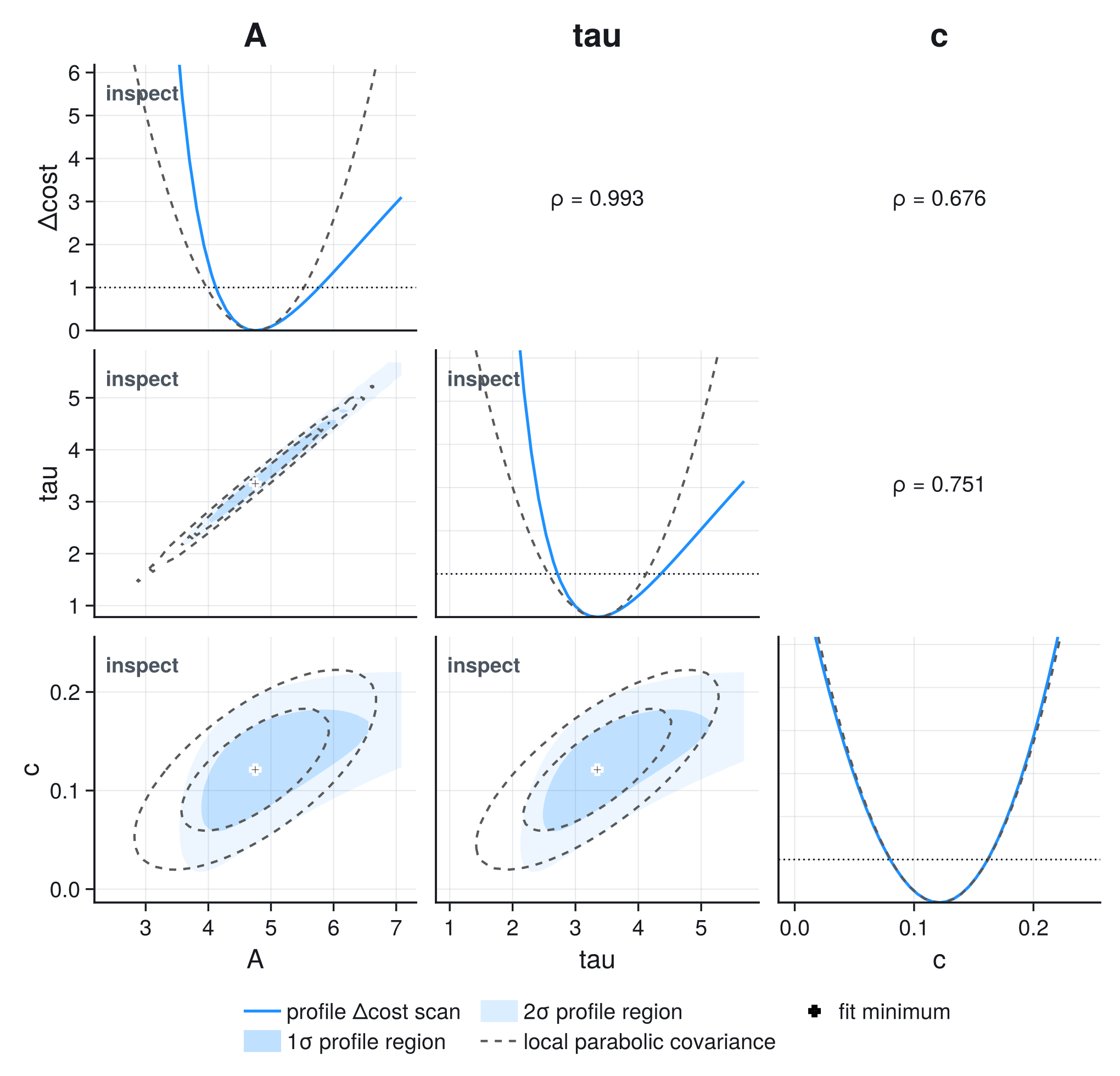
The reading order is mechanical:
- Start in the upper triangle. Correlations near $\pm1$ identify parameter pairs whose local covariance errors are fragile.
- Move to the matching contour panel below the diagonal. If the profiled contour bends away from the dashed local ellipse, the likelihood geometry is not locally Gaussian over the region you intend to report.
- Check the diagonal profile for the parameter you want to quote. If the profile is skewed, use the profile interval instead of $\hat p\pm\sigma$.
Panels labelled inspect correspond to panel_status == :review; a fix label would mark :stop. Here every panel involving $A$ or $\tau$ is flagged, including the baseline pairs with their moderate correlations ($\rho = 0.68$ and $0.75$). But the profiled baseline regions stay close to the local ellipses, while the $A$-$\tau$ panel shows the long curved degeneracy; that contrast makes the amplitude-time-constant block the panel to act on. The independent calibration answers the question from the start of the page: the fitted baseline error of $0.041\ \mathrm{V}$ is half the prior width of $0.08\ \mathrm{V}$, so data and calibration jointly pin $c$ and keep its panels close to elliptical.
Decision In The Laboratory
The contour identifies why the fit is degenerate: the experiment has not observed enough of the saturation plateau. The next actions are specific:
- Extend the acquisition to several time constants ($t$ of order $2\hat\tau$ to $3\hat\tau$, here roughly $7$ to $10\ \mathrm{s}$), where the response approaches the plateau $A + c$.
- Keep the independent baseline measurement, because it prevents $c$ from absorbing part of the early rise.
- Report the profile interval or the profile contour until the added data make the local approximation adequate.
Changing optimizers, tightening tolerances, or adding more early-time points cannot create information about the unseen plateau.
Failure Modes To Inspect
The profile does not reach the requested threshold. Increase the scan range only after checking whether the parameter is practically unidentifiable. A one-sided or unbounded interval may be the correct conclusion.
Profile refits fail. Inspect diagnose(profile_result) or diagnose(contour_result). Failed cells can indicate poor scaling, invalid model evaluations, active bounds, or a secondary minimum.
A narrow contour appears fragmented. Repeat the scan with a denser grid before interpreting isolated regions as secondary minima. This example uses a $121\times121$ grid because the amplitude-timescale region is much narrower across the degeneracy than along it.
The best fit sits on a bound. Do not report a symmetric covariance error as though the cost were unconstrained. State the bound and use a profile-based limit or interval.
The local band looks narrow although the parameters are uncertain. The measured part of the curve can be predicted well while its physical decomposition into $A$ and $\tau$ remains uncertain; prediction uncertainty and parameter identifiability answer different questions.
The effective-variance approximation is questionable. If time uncertainty is large or the model is strongly curved over one $\sigma_t$, the first-order effective-variance treatment is no longer sufficient. Such cases need an explicit errors-in-variables formulation with latent true time values, which this package's effective-variance treatment does not provide; Uncertainty In X states the validity limits.
Next useful pages: Fitting for Practitioners, Profiles and Contours, and XY Uncertainties.