Fit A Peak And Background: LHCb Data
Question: how many entries belong to a peak above a smooth background? Use a Poisson likelihood to estimate its area, compare two peak shapes, and check the signal uncertainty with a profile. DistributionsHEP supplies the mixture, BuildConstructors names its parameters, and NativeMinuit minimizes the same likelihood used for the subsequent profile.
Data And Selection
Source: LHCb collaboration (2017), Matter Antimatter Differences (B meson decays to three hadrons) - Data Files, CERN Open Data Portal, DOI: 10.7483/OPENDATA.LHCB.AOF7.JH09. These are real 2011 proton-proton collision data at 7 TeV, released under CC0-1.0. Each candidate combines three charged tracks. Each track's measured momentum $\vec p_i$ and the assigned kaon mass give an energy $E_i=\sqrt{|\vec p_i|^2+m_K^2}$ (units with $c=1$); the invariant mass of the combination is $m=\sqrt{(\sum_i E_i)^2-|\sum_i \vec p_i|^2}$. When the three tracks come from one $B^\pm\to K^\pm K^+K^-$ decay, energy and momentum conservation make $m$ equal the $B$ mass, smeared by detector resolution; unrelated track combinations have no preferred $m$ and form a smooth, broad background.
LHCb supplied candidates that already pass the trigger (record abstract) and an offline preselection on track momenta, vertex quality and a wide mass window, $5.05<m_{KKK}<6.30\,\mathrm{GeV}/c^2$ under the kaon hypothesis (preselection notebook). We then apply the particle-identification cuts below to the whole MagnetUp file, without random subsampling. LHCb periodically reverses its dipole magnet's polarity, and the record provides one file per polarity; one polarity is enough for this yield estimate, so MagnetDown is not used.
| Choice | Definition |
|---|---|
| File | B2HHH_MagnetUp.root, DecayTree; 3,420,295 candidates |
| Track selection | Every track: ProbK > 0.5, ProbPi < 0.5, isMuon == 0; 9,717 candidates remain |
| Charge | B-plus and B-minus candidates combined |
| Mass | Invariant mass of the three tracks, each assigned $m_K=493.677\,\mathrm{MeV}/c^2$ |
| Fit window | $5200\leq m_{KKK}<5600\,\mathrm{MeV}/c^2$; 7,368 candidates in 80 bins |
The thresholds follow the starting cuts in the LHCb project notebook. ProbK and ProbPi are the detector's per-track particle-identification outputs, scores between 0 and 1 for how kaon-like and how pion-like the track is; isMuon flags tracks matched to the muon system. Requiring three kaon-like, non-pion-like, non-muon tracks suppresses combinations that contain a wrong particle type.
The lower window edge is a physics choice: partially reconstructed $B$ decays, four-body decays with a missed pion or photon, populate the spectrum below the kinematic endpoint $m_B-m_\pi\approx 5140\,\mathrm{MeV}/c^2$ (the ARGUS-shaped component in Fig. 1 of the LHCb publication cited below). Starting at $5200\,\mathrm{MeV}/c^2$ leaves only smooth combinatorial background inside the window, so a single exponential can describe it. A wider window would require an additional background component.
The kaon mass is from the Particle Data Group. Download the UnROOT preparation script to rebuild the histogram from the original file. It checks the file checksum, reconstructs masses and counts every selection step. The histogram below is sufficient to run the fit without downloading ROOT data.
Scope: estimate the signal count in this selected sample and mass window. The fit has 80 Poisson bins and seven free parameters; reading 3.4 million source candidates is a separate data-preparation step.
using ScientificFitting, Distributions, DistributionsHEP, BuildConstructors, Printf
import NativeMinuit  # keep ScientificFitting.profile unambiguous

edges = collect(5200.:5.:5600.)  # MeV/c^2; left-closed, right-open bins
counts = [
    12,16,19,19,24,26,40,64,67,92,152,228,333,419,571,683,
    738,747,711,570,434,291,219,147,88,57,35,36,25,19,16,15,
    13,12,12,3,16,17,13,10,11,11,9,7,10,13,9,12,
    11,6,10,6,8,8,12,13,10,8,8,12,9,7,14,13,
    11,9,7,9,12,7,9,4,15,3,10,9,7,4,3,3,
]
println("Candidates in fit window: ", sum(counts))
Candidates in fit window: 7368Model And Fit
Use two Gaussians with a common center for the peak, and an exponential for the background: random track combinations produce a smooth, slowly falling mass distribution, and the residual panel below checks this choice against the data. A narrow core plus a wider component approximates a mixture of detector resolutions; it represents one peak, not two particles.
For $W=[m_{\mathrm{lo}},m_{\mathrm{hi}})=[5200,5600)$ in $\mathrm{MeV}/c^2$, define
\[\begin{aligned} g(m) &= f\,\mathcal N(m;\mu,\sigma)+(1-f)\,\mathcal N(m;\mu,r\sigma),\\ S(m) &= \frac{g(m)}{\int_W g(u)\,du},\qquad B(m)=\frac{e^{-(m-m_{\mathrm{lo}})/\tau}} {\tau\,[1-e^{-(m_{\mathrm{hi}}-m_{\mathrm{lo}})/\tau}]}. \end{aligned}\]
Both densities vanish outside $W$ and integrate to one inside it. $\mu,\sigma,r,f$ set the peak shape, $\tau$ the background slope, and $N_s,N_b$ the expected signal and background counts in the window. For each bin,
\[\nu_i=N_s\int_{\mathrm{bin}\ i}S(m)\,dm+N_b\int_{\mathrm{bin}\ i}B(m)\,dm, \qquad n_i\sim\operatorname{Poisson}(\nu_i).\]
fit_distribution minimizes $-2\sum_i\log\operatorname{Poisson}(n_i;\nu_i)$. It integrates the densities over each bin, rather than evaluating their heights at bin centers. @with_parameters defines the MassSpectrum model and a companion ConstructorOfMassSpectrum that takes one AdvancedParameter per declared name; each AdvancedParameter declares a name, start and bounds, and ::P inserts the parameter's current value when BuildConstructors builds the distribution.
Start values are read off the histogram: the peak sits near $5284\,\mathrm{MeV}/c^2$ with a width of roughly $15\,\mathrm{MeV}/c^2$. The width-ratio lower bound of 1.05 keeps the second component strictly wider than the core; at $r=1$ the two components would be interchangeable and the fit ill-defined.
@with_parameters(MassSpectrum;
    center::P, width::P, width_ratio::P, core_fraction::P,
    background_scale::P, signal_yield::P, background_yield::P, begin
    peak = MixtureModel(
        [Normal(center, width), Normal(center, width*width_ratio)],
        [core_fraction, 1-core_fraction])
    signal = truncated(peak, 5200., 5600.)
    # Adding 5200. shifts the exponential's support to the window's lower edge;
    # its lower support is already zero, so only truncate its upper end at 400.
    background = 5200. + truncated(Exponential(background_scale); upper=400.)
    ExtendedMixtureModel([signal, background], [signal_yield, background_yield])
end)

constructor = ConstructorOfMassSpectrum(
    AdvancedParameter("center", 5284.; boundaries=(5250.,5310.)),
    AdvancedParameter("width", 14.; boundaries=(3.,30.)),
    AdvancedParameter("width_ratio", 2.; boundaries=(1.05,5.)),
    AdvancedParameter("core_fraction", 0.8; boundaries=(0.05,1.)),
    AdvancedParameter("background_scale", 400.; boundaries=(20.,5000.)),
    AdvancedParameter("signal_yield", 6500.; boundaries=(0.,15000.)),
    AdvancedParameter("background_yield", 1000.; boundaries=(0.,15000.)),
)
result = fit_distribution(constructor, edges, counts;
    solver=NativeMinuitSolver(), tol=1e-3)  # also used for subsequent profile refits

for (name, value, error) in zip(keys(parameter_values(result)), result.params, result.param_stderr)
    @printf("%-18s = %.6g +/- %.3g\n", name, value, error)
end
@printf("Poisson deviance / ndf = %.2f / %d; asymptotic p = %.4f\n",
    result.stats.chi2, result.stats.ndf, result.stats.pvalue)
center = 5284.74 +/- 0.243
width = 14.7468 +/- 1
width_ratio = 1.6733 +/- 0.105
core_fraction = 0.634437 +/- 0.139
background_scale = 531.884 +/- 141
signal_yield = 6484.45 +/- 93.6
background_yield = 883.599 +/- 56.2
Poisson deviance / ndf = 69.44 / 73; asymptotic p = 0.5965The fitted signal is about 6,484 candidates with a local standard error of 94. The Poisson deviance is the likelihood-ratio statistic against a saturated model that reproduces every bin exactly; asymptotically it follows a chi-square distribution with bins minus free parameters degrees of freedom. Here it is 69.44 for $80-7=73$ degrees of freedom, with an approximate $p=0.60$: this check does not detect an overall lack of fit. The fitted centroid lies about $5\,\mathrm{MeV}/c^2$ above the known $B^\pm$ mass; the closing section quantifies this offset. Inspect the residuals next, then test the peak-shape assumption below.
Bounds keep widths and yields physical; they are not priors. The reported errors come from local curvature. fitted_model(result) returns an ExtendedMixtureModel, so plotting or evaluating it does not refit.
What ScientificFitting (SF) adds here: the model itself comes from DistributionsHEP and BuildConstructors; MIGRAD, Minuit's gradient-based minimizer, comes from NativeMinuit.
| Step | Handled by SF |
|---|---|
| Model to likelihood | Integrate component distributions over bins, apply their yields, validate counts and evaluate the Poisson likelihood. |
| Constructor to solver | Transfer names, starts, bounds and fixed values; prepare derivatives and the correct objective scale. |
| Fit to inference | Return covariance, deviance, AIC and named values; retain the model and solver for profile refits and plots. |
NativeMinuit also provides binned likelihoods, HESSE (curvature errors), MINOS (profile-likelihood intervals) and contours; a direct implementation can reach the same result. SF supplies the adapters above and a common result and diagnostics API across solvers. The custom spectrum drawing below remains ordinary Makie code.
Inspect The Spectrum
Evaluate each fitted component over the bin edges. The mean band uses $\sigma_{\nu_i}^2 = J_i\operatorname{Cov}(\hat p)J_i^\mathsf{T}$, where $J_{ij}=\partial\nu_i/\partial p_j$; these are post-fit calculations.
For the data points, $n\pm\sqrt n$ is a poor guide at small counts: an empty bin would even get a zero-width bar. Instead use Garwood intervals for each Poisson mean $\nu$. For confidence level $1-\alpha=0.6827$, they are
\[\nu_{\mathrm{lo}} = \begin{cases} 0, & n=0,\\ \tfrac12\chi^2_{2n,\,\alpha/2}, & n>0, \end{cases} \qquad \nu_{\mathrm{hi}}=\tfrac12\chi^2_{2(n+1),\,1-\alpha/2}.\]
Here $\chi^2_{k,q}$ is the $q$-quantile with $k$ degrees of freedom. The formula inverts the two Poisson tail tests: $\nu_{\mathrm{lo}}$ is the mean for which observing $n$ or more counts has probability $\alpha/2$, and $\nu_{\mathrm{hi}}$ the mean for which observing $n$ or fewer does; means outside the interval would make the observed count a tail event. For $n=0$ this gives $[0,1.84]$, rather than $[0,0]$. Coverage is at least the nominal level because counts are discrete. These bars describe individual bins, not the fitted signal-yield error, and are not weights in the fit. See the central Poisson interval formula.
using ForwardDiff

names = keys(parameter_values(result))
build(p) = build_model(constructor, NamedTuple{names}(Tuple(p)))
component_counts(model) = [n .* diff(cdf.(d, edges))
    for (d, n) in zip(components(model), DistributionsHEP.yields(model))]
signal, background = component_counts(fitted_model(result))
means = signal + background
J = ForwardDiff.jacobian(p -> sum(component_counts(build(p))), result.params)
sigma = sqrt.(vec(sum((J * result.param_covariance) .* J; dims=2)))

# Signed Poisson deviance residuals; a zero count contributes no n*log(n/mu) term.
residual = [sign(n-m)*sqrt(max(2*(m-n+(n==0 ? 0 : n*log(n/m))), 0))
    for (n, m) in zip(counts, means)]

# Central 68.3% Garwood intervals for each bin mean, including empty bins.
tail = (1 - 0.682689492137)/2
lower = [n==0 ? 0. : quantile(Chisq(2n), tail)/2 for n in counts]
upper = [quantile(Chisq(2(n+1)), 1-tail)/2 for n in counts]
centers = (edges[1:end-1] + edges[2:end])/2
step_x = repeat(edges; inner=2)[2:end-1]  # vertical steps at the actual bin edges
@printf("Expected count: %.2f; sum of squared deviance residuals: %.2f\n",
    sum(means), sum(abs2, residual))
Expected count: 7368.05; sum of squared deviance residuals: 69.44Compose two ordinary Makie axes from these arrays; theme, appearance and show_panel are independent options. Change the Makie calls directly to add or restyle elements.
using CairoMakie, LaTeXStrings

"""Draw the fitted bin means and residuals computed above; do not refit."""
function spectrum_figure(; theme=:sans, appearance=:light, show_panel=true)
    pal = plot_palette(theme; appearance)
    return with_theme(plot_theme(theme; appearance)) do
        fig = Figure(size=(show_panel ? 1180 : 900, 740))
        ax = Axis(fig[1,1]; title="LHCb open data: three-kaon mass",
            ylabel="candidates / bin")
        band!(ax, step_x, repeat(means-sigma; inner=2), repeat(means+sigma; inner=2);
            color=(pal.band_color, 0.28), label="local 1-sigma mean band")
        lines!(ax, step_x, repeat(means; inner=2);
            color=pal.fit_color, label="two-width peak + background")
        lines!(ax, step_x, repeat(background; inner=2);
            color=pal.reference_color, linestyle=:dash, label="background")
        errorbars!(ax, centers, counts, counts-lower, upper-counts;
            color=pal.yerr_color, whiskerwidth=pal.error_whiskerwidth)
        scatter!(ax, centers, counts; color=pal.data_color,
            markersize=pal.data_markersize, label="data (68% Poisson intervals)")
        hidexdecorations!(ax; grid=false)

        rx = Axis(fig[2,1]; xlabel=theme==:tex ? L"m_{KKK}\,/(\mathrm{MeV}\,c^{-2})" :
            "three-kaon mass / (MeV/c^2)", ylabel="deviance residual")
        barplot!(rx, centers, residual; width=0.8 .* diff(edges), color=pal.fit_color)
        hlines!(rx, [0.]; color=pal.stats_color)
        hlines!(rx, [-2., 2.]; color=pal.reference_color, linestyle=:dash)
        linkxaxes!(ax, rx)
        xlims!(ax, first(edges), last(edges))
        ylims!(ax, 0, 1.08maximum(upper))
        rowsize!(fig.layout, 1, Auto(3))
        rowsize!(fig.layout, 2, Auto(1))

        if show_panel
            p, e = result.params, result.param_stderr
            labels = theme==:tex ? Any[
                LaTeXString(@sprintf("N_s = %.0f \\pm %.0f", p[6], e[6])),
                LaTeXString(@sprintf("N_b = %.0f \\pm %.0f", p[7], e[7])),
                LaTeXString(@sprintf("\\mu = %.2f \\pm %.2f\\;\\mathrm{MeV}/c^2", p[1], e[1])),
                LaTeXString(@sprintf("\\sigma = %.2f \\pm %.2f\\;\\mathrm{MeV}/c^2", p[2], e[2])),
            ] : Any[@sprintf("signal = %.0f +/- %.0f candidates", p[6], e[6]),
                @sprintf("background = %.0f +/- %.0f candidates", p[7], e[7]),
                @sprintf("centroid = %.2f +/- %.2f MeV/c^2", p[1], e[1]),
                @sprintf("core width = %.2f +/- %.2f MeV/c^2", p[2], e[2])]
            plot_info_panel!(fig[1:2,2]; theme, appearance, legend_source=ax,
                title="Window-conditional fit", parameter_lines=labels,
                statistic_lines=[@sprintf("D / ndf = %.2f / %d", result.stats.chi2, result.stats.ndf),
                    @sprintf("asymptotic p = %.3f", result.stats.pvalue)])
        else
            Legend(fig[3,1], ax; nbanks=2, tellwidth=false)
        end
        resize_plot_to_layout!(fig; minimum_axis_size=(600, nothing))
        fig
    end
end

figure = spectrum_figure(; theme=:sans, show_panel=true)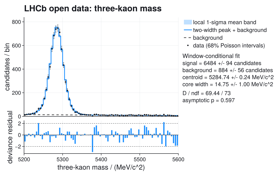
The lower axis shows signed Poisson deviance residuals: look for runs of bins that the fit consistently over- or underestimates. The shaded mean band contains parameter uncertainty, not the additional fluctuation of future counts.
Check Shape Dependence
Set the core fraction to one and fix the now-unused width ratio: the same constructor becomes a single-Gaussian model.
single = deepcopy(constructor)
BuildConstructors.update!(single, (core_fraction=1.,))
fix!(single, (:core_fraction, :width_ratio))
single_result = fit_distribution(single, edges, counts;
    solver=NativeMinuitSolver(), tol=1e-3)
for (label, fit) in (("one width", single_result), ("two widths", result))
    @printf("%-11s  Ns = %.1f +/- %.1f   D/ndf = %.2f/%d   p = %.4f\n",
        label, fit.params[6], fit.param_stderr[6], fit.stats.chi2, fit.stats.ndf, fit.stats.pvalue)
end
@printf("AIC(one) - AIC(two) = %.2f\n", single_result.stats.aic-result.stats.aic)
one width Ns = 6336.1 +/- 85.9 D/ndf = 101.96/75 p = 0.0209
two widths Ns = 6484.5 +/- 93.6 D/ndf = 69.44/73 p = 0.5965
AIC(one) - AIC(two) = 28.53The two-width model describes these data better: the deviance falls from 101.96 to 69.44, and the fitted signal increases by about 148 candidates. This supports allowing a wider resolution component; it does not identify a second physical signal. The AIC difference is meaningful because both fits use the same data and the same likelihood normalization (Model Comparison With AIC And BIC).
The yield shift measures sensitivity to the peak model, not an independent error to add in quadrature. The p-values are approximate, especially in sparse bins. Do not assign the standard two-parameter likelihood-ratio significance to the improvement: the single-Gaussian model sets the wide component's weight $1-f$ to zero, and at that boundary the width ratio $r$ has no effect on the model, so the chi-square calibration of the likelihood-ratio test does not apply.
See The Yield Uncertainty
Could a different peak width or background level change the signal count? Fix $N_s$ at a series of trial values and refit the other six parameters. Plot the resulting cost increase against the local covariance parabola:
scan = profile(result, 6; nsigma=2.5, npoints=31, on_failure=:throw)
interval = profile_interval(scan)
@printf("Ns profile interval at delta(-2 log L)=1: [%.1f, %.1f]\n",
    interval.lower, interval.upper)
profile_options = (local_sigma=result.param_stderr[6],
    title="Uncertainty of the signal count", xlabel="signal count Ns",
    ylabel="Delta (-2 log L)")
profile_figure = plot_profile(scan; profile_options...)
Ns profile interval at delta(-2 log L)=1: [6391.5, 6578.6]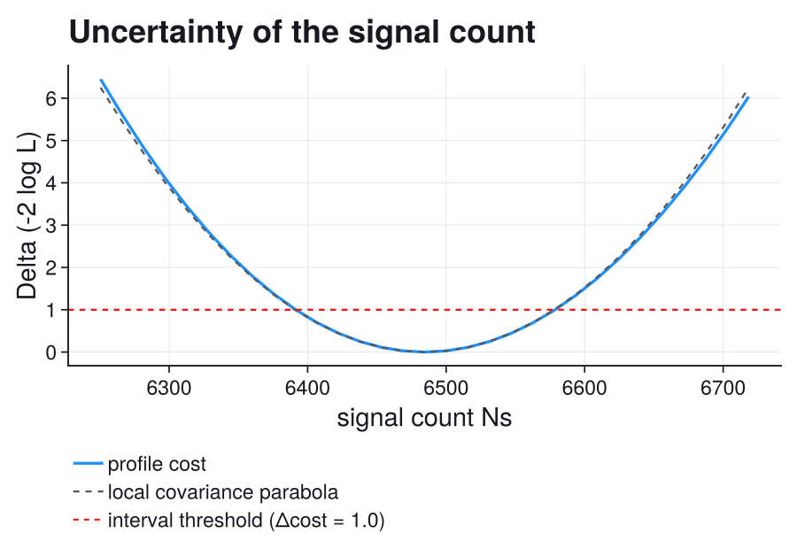
The curve is close to a parabola in the relevant range. Its crossings at $\Delta(-2\log L)=1$ give about $[6391,6579]$ candidates, consistent with $N_s\pm94$. This is an approximate one-parameter 68.3% interval, with the shape and background refitted rather than frozen (why a profile is not a slice).
To see the trade-off between signal and background, vary both yields together. At each grid point, refit the five shape parameters:
joint = ScientificFitting.contour(result, 6, 7;
    npoints=25, nsigma=3, on_failure=:throw)
contour_options = (local_covariance=result.param_covariance,
    local_center=result.params[[6, 7]], title="Signal and background counts",
    xlabel="signal count Ns", ylabel="background count Nb")
contour_figure = plot_contour(joint; contour_options...)
@printf("Local correlation of signal and background yields: %.3f\n",
    result.param_correlation[6,7])
Local correlation of signal and background yields: -0.432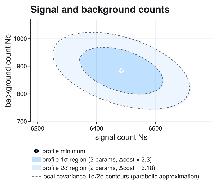
The filled regions use $\Delta(-2\log L)=2.30,6.18$ for approximate joint 68.3% and 95.45% coverage; dashed ellipses show the local covariance approximation. Their tilt shows how increasing one yield can be compensated by decreasing the other; one- and two-parameter thresholds differ (Profiles And Contours). Neither calculation includes uncertainty from choosing the wrong peak or background shape.
The independent numerical check, run from the repository with NumPy, SciPy and iminuit, compares both fits and the signal-yield MINOS interval: Minuit's algorithm for the same interval as profile_interval above, the crossings of the profiled $-2\log L$ at $\Delta(-2\log L)=1$, located by its own iteration instead of a grid of refits. Hidden assertions in this page's source pin the deviance of both fits, the two-width parameters and errors, and the signal-yield interval to values cross-checked against that script; the agreement tests the numerical implementation of this model.
What The Yield Measures
$N_s$ counts the fitted peak in this selection and window, before efficiency corrections. The LHCb publication instead fits charges separately, uses a different selection and more detailed signal and background shapes, then corrects detector and production effects to measure CP asymmetry. Its $22\,119\pm164$ yield is therefore not a target for this fit.
We do not exclude candidates whose two-kaon mass matches a charm meson, as the publication does, so decays through an intermediate charm meson, $B^\pm\to\bar D^0K^\pm$ with $\bar D^0\to K^+K^-$ and the same three-kaon final state, can also contribute to the peak.
The fitted centroid, $5284.74\pm0.24\,\mathrm{MeV}/c^2$, lies about $5\,\mathrm{MeV}/c^2$ (0.1%) above the PDG $B^\pm$ mass of $5279.41\pm0.07\,\mathrm{MeV}/c^2$. The raw counts peak in the same bins, so the offset is a property of these data, not of the fit: no momentum-scale calibration is applied here or documented for the open-data ntuple (a 0.1% scale shift moves the reconstructed mass by about this amount), and residual misidentified $B^\pm\to\pi^\pm K^+K^-$ decays can enter with an upward-shifted mass. The centroid locates the peak in this selection and window; it is not a measurement of the $B^\pm$ mass.