Damped Oscillator: When A Good-Looking Fit Is Wrong

A dense nonlinear fit can look almost perfect while its residuals reject the model. This workflow uses a laboratory recording of a freely decaying mechanical oscillator to answer two questions:

1. What damping rate and oscillation frequency describe the record?
2. Is a constant-frequency damped oscillator an adequate model?

Question

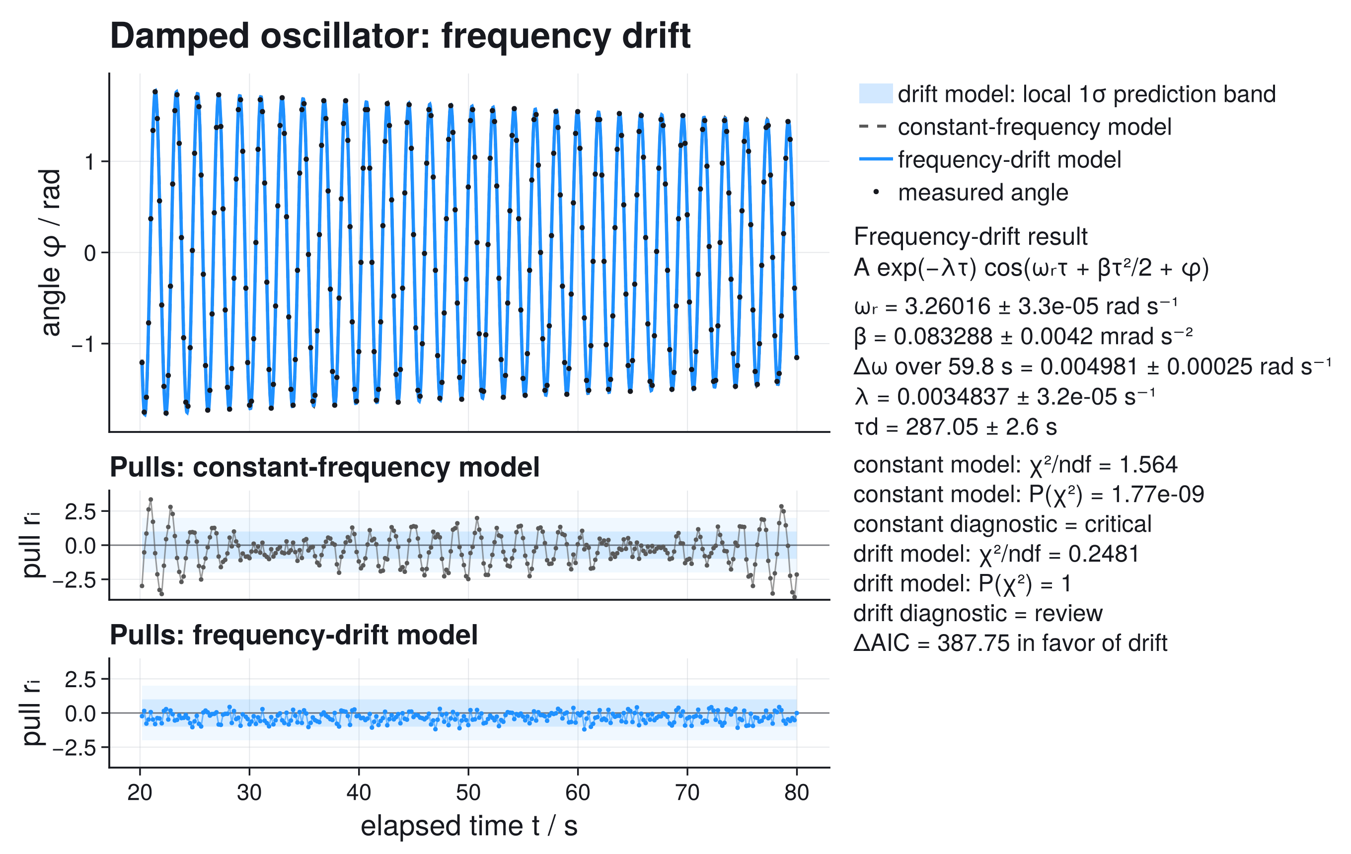
The main panel alone barely distinguishes the two models. The pull panels — each point's residual divided by its expected standard deviation, defined below — do: the constant-frequency model leaves coherent deviations, while a weak frequency drift removes most of that structure.

The Measurement

Data provenance. The record is the author's own laboratory measurement of the free decay of a Pohl torsion pendulum (a rotating-wheel torsion oscillator, a standard undergraduate-laboratory apparatus). It ships with this repository as examples/data/damped_oscillator/pohl_wheel_free_decay.csv under the repository's MIT license.

The source acquisition recorded the angular displacement at 50 Hz. The distributed CSV keeps every tenth raw sample between 20.18 s and 79.98 s, giving 300 points at approximately 5 Hz. The values were neither smoothed nor interpolated.

The angle was reconstructed from a path displacement measured at the instrument radius of 91.9 mm. The acquisition analysis assigned a 1 mm path-length uncertainty, so the angle uncertainty stored in the file is

\[\sigma_\phi = \frac{1\ \mathrm{mm}}{91.9\ \mathrm{mm}} = 0.0108814\ \mathrm{rad}.\]

This is an instrument-based assignment, not a standard deviation estimated from repeated decay records. The analysis keeps it unchanged and assigns a 0.5 ms standard timestamp uncertainty from the acquisition timing resolution, so both x and y uncertainty enter the fit. Whether an independent Gaussian model is compatible with those assignments is a result to diagnose.

Model: Start With The Physical Baseline

For a torsion oscillator with moment of inertia $\Theta$, damping coefficient $b$, and torsional stiffness $D$, the linear equation of motion is

\[\Theta\ddot\phi+b\dot\phi+D\phi=0.\]

In the underdamped regime ($\lambda^2 < D/\Theta$, so the oscillation persists) the solution is

\[\phi(t) = A_\mathrm{ref} e^{-\lambda \tau} \cos\!\left(\omega_\mathrm{ref}\tau+\phi_\mathrm{ref}\right), \qquad \tau=t-t_\mathrm{ref}.\]

The parameters are:

• $A_\mathrm{ref}$: amplitude at the reference time,
• $\lambda$: exponential damping rate,
• $\omega_\mathrm{ref}$: damped angular frequency,
• $\phi_\mathrm{ref}$: phase at the reference time.

The time coordinate is centered at the middle of the record: without centering, phase and frequency must compensate for a large arbitrary time origin and become more strongly correlated.

The damping time is the derived quantity

\[\tau_d = \frac{1}{\lambda},\]

the time over which the oscillation amplitude falls by a factor $e$.

For the constant-coefficient model,

\[\lambda=\frac{b}{2\Theta}, \qquad \omega_\mathrm{ref} =\sqrt{\frac{D}{\Theta}-\lambda^2}.\]

Diagnostics: Fit and Diagnose the Baseline

The fit uses a Gaussian likelihood with the assigned angle uncertainty and effective-variance propagation of timestamp uncertainty (Uncertainty In X). solver=:ipnewton selects the interior-point solver, which handles the box bounds directly and converges cleanly from every start used here. The explicit tol=1e-7 is a numerical stopping tolerance; tightening it further does not change the reported digits.

For this diagonal uncertainty model, the plotted pulls are

\[r_i =\frac{\phi_i-f(t_i,p)} {\sqrt{\sigma_{\phi,i}^2+ \left(\partial f/\partial t\right)_i^2\sigma_{t,i}^2}}.\]

Their expected behavior under a correct model is described in Residuals And Pulls.

Phase-periodic models have repeated local minima. The two explicit initial_guesses are always tried in addition to p0, and the fit keeps the candidate with the lowest cost; this does not prove that the minimum is global. (The multistart keyword sets a total candidate budget and would only add generated starts beyond the explicit list.)

The start values are read off the record: $A_\mathrm{ref}$ from the envelope near mid-record, $\omega_\mathrm{ref} = 2\pi/T$ from the visible period $T \approx 1.93\ \mathrm{s}$, $\phi_\mathrm{ref} = 0$ as a neutral phase start, and $\lambda$ from the rough amplitude ratio between the two ends of the record.

using ScientificFitting

function load_damped_oscillator(path)
    rows = readlines(path)[2:end]
    parsed = [parse.(Float64, split(row, ",")) for row in rows if !isempty(strip(row))]
    return (
        time=[row[1] for row in parsed],
        angle=[row[2] for row in parsed],
        sigma_angle=[row[3] for row in parsed],
    )
end

data = load_damped_oscillator(
    "examples/data/damped_oscillator/pohl_wheel_free_decay.csv",
)
time = data.time
angle = data.angle
sigma_angle = data.sigma_angle
sigma_time = fill(0.0005, length(time))
time_reference = (minimum(time) + maximum(time)) / 2

constant_frequency_model(t, p) = @. p[1] * exp(-p[4] * (t - time_reference)) *
                                     cos(p[2] * (t - time_reference) + p[3])

constant_result = fit_model(
    constant_frequency_model,
    time,
    angle;
    p0=[1.6, 3.26, 0.0, 0.0035],
    sigma_y=sigma_angle,
    sigma_x=sigma_time,
    bounds=([0.0, 2.0, -20.0, 0.0], [5.0, 5.0, 20.0, 0.05]),
    initial_guesses=[
        [1.8, 3.20, 2.0, 0.0020],
        [1.5, 3.35, -2.0, 0.0060],
    ],
    solver=:ipnewton,
    maxiters=3000,
    tol=1e-7,
)

println(report_text(
    constant_result;
    parameter_names=["A_ref", "omega_ref", "phi_ref", "lambda"],
))
println(diagnostic_dashboard_text(constant_result))

Fit report
backend = optimization
converged = true
iterations = 43
message = Success

Parameters:
  A_ref = 1.60616 +/- 0.00090
  omega_ref = 3.260100 +/- 0.000033
  phi_ref = -0.76320 +/- 0.00057
  lambda = 0.003485 +/- 0.000032

Statistics:
  cost = gaussian_likelihood
  cost_min = -1689.59
  minus2loglik_min = -1689.59
  chi2 = 462.933
  ndf = 296
  chi2/ndf = 1.56396
  pvalue = 1.76695e-9
  AIC = -1681.59
  BIC = -1666.77
Fit diagnostic dashboard
status = critical - fix before use
critical = 1, warning = 3, info = 0
1 critical issue(s), 3 warning(s). Fix the issue before using this result for conclusions.

Next actions:
  1. Under the stated assumptions this fit is statistically implausible. Inspect residuals and the uncertainty model.
  2. Use a covariance model, inspect acquisition order/time dependence, or fit a model with the missing systematic component.
  3. Inspect residuals near the largest pull. One point may dominate the result or the uncertainty model may be too optimistic.
  4. Look for missing model structure, drift, a calibration offset, or correlated uncertainty in that interval.

The fit converges and gives plausible parameter values, but convergence does not validate the model.

For this fit,

\[\frac{\chi^2}{\mathrm{ndf}} = 1.564, \qquad P(\chi^2) = 1.77\times 10^{-9},\]

with $\mathrm{ndf} = 300$ points $- \, 4$ free parameters $= 296$ (Degrees Of Freedom).

Under the stated independent Gaussian uncertainty model, residuals this incompatible would be extraordinarily unlikely (Goodness Of Fit), and the dashboard status is critical.

The first pull panel explains why: the deviations change coherently over time instead of scattering around zero.

Test A Specific Missing Effect

A slowly changing oscillation frequency produces an accumulating phase error. The smallest useful extension adds a linear frequency drift:

\[\phi(t) = A_\mathrm{ref}e^{-\lambda\tau} \cos\!\left( \omega_\mathrm{ref}\tau + \frac{1}{2}\beta\tau^2 + \phi_\mathrm{ref} \right),\]

where

\[\omega(t)=\frac{\mathrm{d}}{\mathrm{d}t} \left( \omega_\mathrm{ref}\tau+\frac{1}{2}\beta\tau^2+\phi_\mathrm{ref} \right) =\omega_\mathrm{ref}+\beta\tau.\]

The new parameter $\beta$ has units $\mathrm{rad\,s^{-2}}$. This is a phenomenological test, not yet a claim about mechanism: amplitude-dependent stiffness, temperature drift, or a small timing-scale error could all produce accumulated phase structure.

frequency_drift_model(t, p) = @. p[1] * exp(-p[4] * (t - time_reference)) *
                                  cos(
    p[2] * (t - time_reference) +
    0.5 * p[5] * (t - time_reference)^2 +
    p[3],
)

drift_result = fit_model(
    frequency_drift_model,
    time,
    angle;
    p0=[1.6, 3.26, 0.0, 0.0035, 0.0],
    sigma_y=sigma_angle,
    sigma_x=sigma_time,
    bounds=([0.0, 2.0, -20.0, 0.0, -0.01], [5.0, 5.0, 20.0, 0.05, 0.01]),
    initial_guesses=[
        [1.8, 3.20, 2.0, 0.0020, 0.0001],
        [1.5, 3.35, -2.0, 0.0060, -0.0001],
    ],
    solver=:ipnewton,
    maxiters=4000,
    tol=1e-7,
)

println(report_text(
    drift_result;
    parameter_names=["A_ref", "omega_ref", "phi_ref", "lambda", "beta"],
))
println(diagnostic_dashboard_text(drift_result))

Fit report
backend = optimization
converged = true
iterations = 33
message = Success

Parameters:
  A_ref = 1.60608 +/- 0.00090
  omega_ref = 3.260157 +/- 0.000033
  phi_ref = -0.77561 +/- 0.00085
  lambda = 0.003484 +/- 0.000032
  beta = 8.32878e-5 +/- 4.21994e-6

Statistics:
  cost = gaussian_likelihood
  cost_min = -2079.34
  minus2loglik_min = -2079.34
  chi2 = 73.1838
  ndf = 295
  chi2/ndf = 0.248081
  pvalue = 1.0
  AIC = -2069.34
  BIC = -2050.82
Fit diagnostic dashboard
status = review - inspect diagnostics
critical = 0, warning = 1, info = 0
1 warning(s). Inspect before trusting uncertainties or conclusions.

Next actions:
  1. The uncertainties may be too large, correlations may be ignored, or the data may not be independent.

Read The Comparison, Not Just The Better Curve

The fitted drift and damping parameters are

\[\beta = (8.33 \pm 0.42)\times 10^{-5}\ \mathrm{rad\,s^{-2}},\]

\[\lambda = (3.484 \pm 0.032)\times 10^{-3}\ \mathrm{s^{-1}}, \qquad \tau_d = (287.1 \pm 2.6)\ \mathrm{s}.\]

The quoted damping-time uncertainty is the local first-order propagation $\sigma_{\tau_d}=\sigma_\lambda/\lambda^2$ and inherits the limitations of the local $\lambda$ covariance.

Across the recorded interval, the fitted angular frequency changes by

\[\Delta\omega = \beta(t_{\max}-t_{\min}) = (4.98 \pm 0.25)\times 10^{-3}\ \mathrm{rad\,s^{-1}}.\]

That change is only about 0.15% of $\omega_\mathrm{ref}$, yet its phase effect accumulates over many cycles and becomes obvious in the pulls.

The two fits share observations and likelihood, so their AIC values are comparable (Model Comparison With AIC And BIC). The drift model improves AIC by approximately 388 despite adding only one parameter: the constant-frequency model is inadequate for this record.

The drift model removes the coherent phase pattern, but its pulls are now much narrower than a unit Gaussian:

\[\frac{\chi^2_\mathrm{drift}}{\mathrm{ndf}}=0.248, \qquad P(\chi^2_\mathrm{drift})\approx 1.\]

This suggests a conservative assigned angle uncertainty, non-independent neighboring samples, or both; the dashboard status is review. The data strongly support an accumulated phase correction, but the local parameter errors should not be treated as final until the uncertainty model has been validated with instrument specifications or repeated decay records.

What The Band Means

The main panel shows the drift model's local 1σ prediction band. It combines:

\[\sigma_\mathrm{pred}^2(t) = J_p(t)\,\mathrm{Cov}(p)\,J_p^\mathsf{T}(t) + \sigma_\phi^2 + \left(\frac{\partial f}{\partial t}\sigma_t\right)^2,\]

where $J_p(t)=\left(\partial f/\partial A_\mathrm{ref},\ \partial f/\partial\omega_\mathrm{ref},\ \partial f/\partial\phi_\mathrm{ref},\ \partial f/\partial\lambda,\ \partial f/\partial\beta\right)$ is the row vector of drift-model derivatives with respect to the fitted parameters, evaluated at time $t$ and at the fitted values, and $\mathrm{Cov}(p)$ is the fitted parameter covariance matrix (drift_result.param_covariance). $\sigma_\phi$ and $\sigma_t$ are the assigned angle and timestamp uncertainties from The Measurement above.

The band is narrow compared with the full oscillation amplitude and difficult to judge in the main panel; the pull panels display the same uncertainty scale directly: the darker region is $\pm1\sigma$ and the lighter region is $\pm2\sigma$.

The band uses the local covariance matrix and is conditional on the fitted model; it does not include uncertainty about whether frequency drift is the correct physical explanation.

Complete Reproducible Figure

The tracked script contains the complete fit, diagnostics, derived quantities, prediction-band propagation, and compound Makie figure:

julia --project=docs examples/gallery/08_damped_oscillator_decay.jl

It prints both diagnostic dashboards and writes examples/output/08_damped_oscillator_decay.png.

What To Do Before Reporting A Physical Result

For a critical analysis, the next work is experimental:

1. Determine whether neighboring angle samples share acquisition or filtering correlations.
2. Validate the supplied angle uncertainty against repeated measurements or stationary segments.
3. Test whether the frequency drift repeats in independent decay records.
4. Compare the drift model with a physically motivated nonlinear-oscillator or friction model.
5. Refit after defining the correct covariance model, then reassess pulls and parameter intervals.

The baseline model fails; frequency drift explains the dominant structure; the uncertainty model still requires investigation.

To model shared sample noise explicitly, revisit Full Covariance. Continue with Photoelectric Work Function for a derived physical quantity obtained from two fitted regimes.