XY Uncertainties
This controlled calibration workflow shows what changes when the independent variable has uncertainty too: if the model is steep enough, uncertainty in $x$ contributes to the statistical cost and to the fitted parameter errors.
Question
A voltage sensor is calibrated by measuring stage position $x_\mathrm{meas}$ in millimetres and sensor response $U_\mathrm{meas}$ in volts. Both instruments have finite resolution. The measurements are modeled as
\[U = m x + b;\]
the scientific question is the sensitivity $m$ and offset $b$ with realistic uncertainties on both. Ignoring the $x$ uncertainty treats the measured abscissa as exact and usually yields parameter errors that are too small.
Data
The data are listed literally in the code below; the scatter is fixed in the listed numbers, and no random generator runs when the page is built. The uncertainties are:
- $\sigma_x = 0.05\,\mathrm{mm}$ for every measured position,
- $\sigma_U = 0.033\,\mathrm{V}$ for every measured voltage.
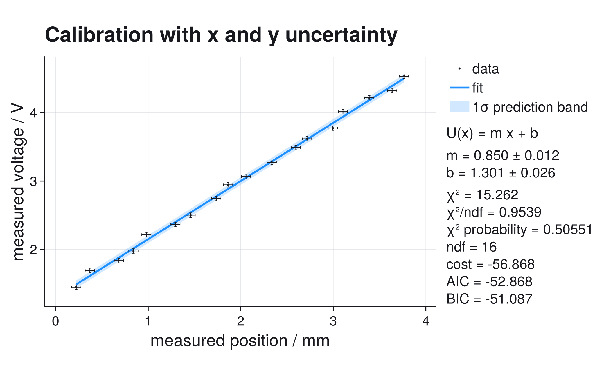
The error bars in the plot correspond to these 1σ standard uncertainties; the 1σ prediction band combines the fitted parameter uncertainty with the effective observation noise $\sigma_\mathrm{eff}$ (both error components, defined below).
Model and Cost
An uncertainty in $x$ enters the vertical residual through the local model slope; Uncertainty In X derives the effective variance $\sigma_{\mathrm{eff},i}^2=\sigma_{y,i}^2+\left(\partial_x f(x_i,p)\,\sigma_{x,i}\right)^2$. For a straight line this becomes
\[\sigma_{\mathrm{eff},i}^2 = \sigma_y^2 + (m\sigma_x)^2.\]
The size of the effect is easy to estimate before fitting: with $m\approx0.85\,\mathrm{V\,mm^{-1}}$ and $\sigma_x=0.05\,\mathrm{mm}$, the x-resolution contributes about $m\sigma_x\approx0.043\,\mathrm{V}$ — larger than $\sigma_U=0.033\,\mathrm{V}$ — so fitting as if x were exact would understate the parameter uncertainty.
ScientificFitting uses this effective variance when sigma_x is supplied. It is a local first-order approximation for smooth models and moderate x errors, not a full errors-in-variables model.
Fit
This is the complete code for the documentation example:
using CairoMakie
using ScientificFitting

# Both coordinates are measured. sigma_x and sigma_U are standard
# uncertainties, not visual-only error-bar lengths.
x_measured = [0.2240, 0.3698, 0.6835, 0.8413, 0.9811, 1.2948,
              1.4586, 1.7364, 1.8641, 2.0579, 2.3356, 2.5954,
              2.7172, 2.9949, 3.1047, 3.3885, 3.6362, 3.7640]
U_measured = [1.450, 1.694, 1.838, 1.978, 2.218, 2.366,
              2.502, 2.746, 2.946, 3.066, 3.274, 3.490,
              3.618, 3.774, 4.014, 4.218, 4.322, 4.530]
sigma_x = fill(0.050, length(x_measured))
sigma_U = fill(0.033, length(x_measured))

line_model(x, p) = @. p[1] * x + p[2]

result = fit_model(
    line_model,
    x_measured,
    U_measured;
    p0=[0.8, 1.2],
    sigma_y=sigma_U,
    sigma_x=sigma_x,
)

plot_fit(
    result;
    title="Calibration with x and y uncertainty",
    model_label="U(x) = m x + b",
    xlabel="measured position",
    xunit="mm",
    ylabel="measured voltage",
    yunit="V",
    parameter_names=["m", "b"],
    band=:prediction,
    nsigma=1,
    band_label="1σ prediction band",
    show_legend=true,
    stats_position=:right,
    stats_mode=:full,
    # Smaller markers keep the x and y error bars visible.
    style=FitPlotStyle(data_markersize=5),
    filename="xy_uncertainties.pdf",
)

println(report_text(result; parameter_names=["m", "b"]))
println(diagnostic_dashboard_text(result))Fit report backend = optimization converged = true iterations = 7 message = Success Parameters: m = 0.850 +/- 0.012 b = 1.301 +/- 0.026 Statistics: cost = gaussian_likelihood cost_min = -56.8681 minus2loglik_min = -56.8681 chi2 = 15.2624 ndf = 16 chi2/ndf = 0.953897 pvalue = 0.505514 AIC = -52.8681 BIC = -51.0874 Fit diagnostic dashboard status = ok - no immediate issue critical = 0, warning = 0, info = 0 No major diagnostic issues detected by the current checks. No next action required by the current diagnostic checks.
The report's backend line names the numerical route that solved the fit; it is selected through the solver keyword of fit_model.
cost_min is the full $-2\log L$, which adds the normalization terms $\sum_i \ln(2\pi\sigma_{\mathrm{eff},i}^2)$ to $\chi^2$; with $\sigma_\mathrm{eff}\approx0.054\,\mathrm{V}$ these terms are negative, so a negative cost is expected (see The Cost Convention).
The visible band is a 1σ prediction band; it is not a profile interval and not a confidence band for the mean line alone.
Diagnostics
Checks before moving to more complicated models:
- Compare the result with and without
sigma_x: the central value should not jump wildly, but the parameter uncertainty should increase. - Plot the residuals against $x$ and inspect them for structure; a systematic trend or curvature — rather than random scatter around zero — means the line may be an incomplete model even with correctly propagated error bars.
- Check $\chi^2/\mathrm{ndf}$ and the p-value; the sample-size-aware reading is in Goodness Of Fit.
- For steep nonlinear models, run profiles or a more explicit measurement-error model before trusting local symmetric errors.
The dashboard reports status = ok - no immediate issue: convergence, goodness-of-fit, residual structure, and local covariance pass its first-line checks. Whether the effective-variance approximation is the correct physical model still depends on how the two instruments produce their errors.
Interpretation
The fitted slope is the calibration sensitivity, and the intercept is the offset. Because $\sigma_x$ contributes through the slope, the uncertainty of $m$ and $b$ depends on the fitted model itself; x errors cannot be added later by drawing larger horizontal error bars on a finished plot.
For the dataset shown here, the fitted sensitivity and offset are
\[m = (0.850 \pm 0.012)\,\mathrm{V\,mm^{-1}}, \qquad b = (1.301 \pm 0.026)\,\mathrm{V}.\]
Under the stated independent Gaussian resolution model, $\chi^2/\mathrm{ndf}=0.954$ and the p-value $p=0.506$ are statistically unremarkable.
The reported covariance is local curvature after the effective-variance approximation has been applied; if the approximation is poor, it can be precise but statistically misleading.
What Can Go Wrong
Do not use sigma_x as a visual-only option: it changes the cost function. For horizontal error bars without statistical weight, draw them in a custom plot instead.
Do not use effective variance for discontinuous or kinked models; a first-order derivative approximation is not meaningful at a threshold, clipping point, or sharp regime switch.
Large x errors, unknown true x values that must be estimated alongside the parameters, and calibration transfer problems may require a full measurement model with nuisance parameters or a structured covariance description.
Next useful pages: Full Covariance, Damped Oscillator, and Full Gaussian Likelihood.