Full Covariance
This workflow fits a detector-voltage transient when neighboring samples share readout noise. A covariance matrix tells the fit which residual patterns are plausible together.
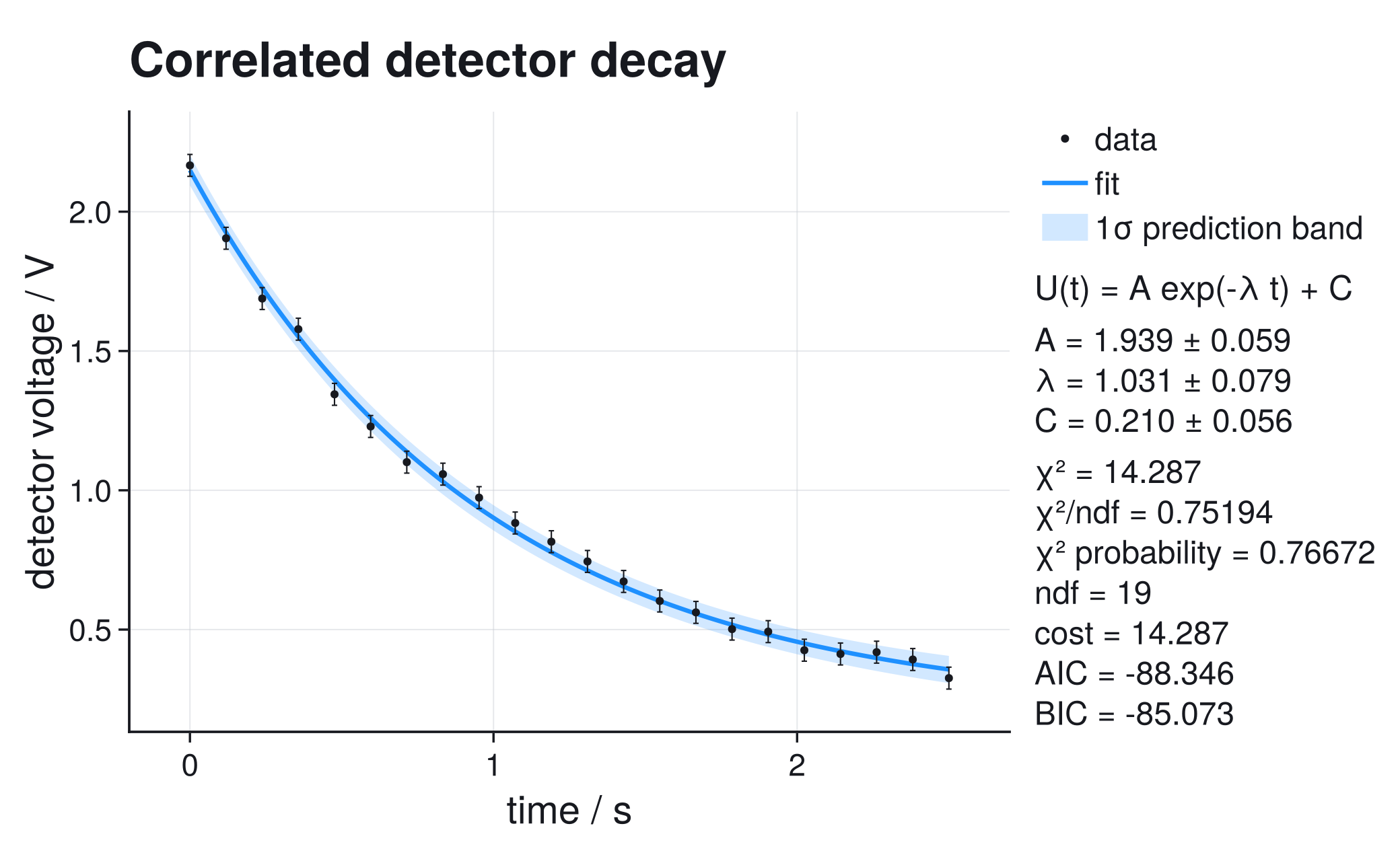
Question
A decaying voltage is sampled repeatedly with the same readout chain, so baseline drift, electronics, or smoothing in the acquisition system affects several samples at once. The scientific question is:
\[U(t) = A e^{-\lambda t} + C,\]
where $t$ is the time since the start of the record in seconds, $A$ and $C$ are voltages, and the positive decay rate $\lambda$ has units $\mathrm{s^{-1}}$.
If the correlations are ignored, the fit can look artificially precise: many small residuals in the same direction carry less independent information than the same number of uncorrelated residuals.
Data and Covariance
The record below is a controlled teaching record, not archival experimental data: it is constructed so that the covariance model given next describes its noise, and the three noise parameters are known by construction rather than estimated. Each point has two kinds of uncertainty:
- a local statistical part, such as readout noise that changes independently from sample to sample,
- a shared part, such as baseline drift, temperature drift, filtering, or electronics noise that affects nearby samples in similar directions.
The compact model used here keeps those contributions separate; the covariance $V_{ij}$ between the voltage measurements at times $t_i$ and $t_j$ is modeled as
\[V_{ij} = \sigma_\mathrm{stat}^2\,\delta_{ij} + \sigma_\mathrm{corr}^2 \exp\!\left(-\frac{|t_i-t_j|}{\tau_\mathrm{corr}}\right).\]
The Kronecker delta $\delta_{ij}$ puts the local variance only on the diagonal; the exponential term is the disturbance shared by nearby samples. In this record,
\[\sigma_\mathrm{stat}=0.018\,\mathrm{V},\qquad \sigma_\mathrm{corr}=0.035\,\mathrm{V},\qquad \tau_\mathrm{corr}=0.28\,\mathrm{s}.\]
For real data these three numbers are inputs to the fit, not outputs of it: they come from characterizing the acquisition chain, for example from the sample variance of repeated baseline records and the autocorrelation of signal-free samples.
The marginal uncertainty of one point is $\sqrt{\sigma_\mathrm{stat}^2+\sigma_\mathrm{corr}^2}=0.0394\,\mathrm{V}$, but adjacent points (spacing $\Delta t = 0.119\,\mathrm{s}$) have total correlation coefficient $\rho = \sigma_\mathrm{corr}^2\,e^{-\Delta t/\tau_\mathrm{corr}}/(\sigma_\mathrm{stat}^2+\sigma_\mathrm{corr}^2)\approx0.52$ — smaller than the shared term's own $e^{-\Delta t/\tau_\mathrm{corr}}\approx0.65$ because the independent readout variance dilutes it. Two neighboring residuals with the same sign are therefore less surprising than for independent $0.0394\,\mathrm{V}$ errors.
This is a useful first model when the acquisition chain has a finite memory: baseline estimates, smoothing filters, thermal drift, or slowly varying electronics offsets all create nearby residuals with the same sign. A constant calibration scale error is a different mechanism and belongs in a separate nuisance parameter or in the final-result propagation, not in this short-range covariance; the representation table in Correlated Measurements And Whitening maps mechanisms to representations.
A three-sample sketch shows what the two terms do:
\[V = \underbrace{\sigma_\mathrm{stat}^2 \begin{pmatrix}1&0&0\\0&1&0\\0&0&1\end{pmatrix}}_{\text{independent readout}} + \underbrace{\sigma_\mathrm{corr}^2 \begin{pmatrix}1&\rho_1&\rho_2\\\rho_1&1&\rho_1\\\rho_2&\rho_1&1\end{pmatrix}}_{\text{shared disturbance}}, \qquad \rho_k=e^{-\Delta t_k/\tau_\mathrm{corr}},\]
where $\Delta t_k$ is the time separation between samples $k$ steps apart; the sketch assumes uniform spacing, as in the record below.
Model and Cost
With a full covariance matrix $V$, the Gaussian cost is the quadratic form $\chi^2 = r^\mathsf{T} V^{-1} r$ with $r_i = y_i - f(t_i,p)$, where $y_i$ is the measured voltage at time $t_i$, $f$ is the model $U(t)$ above, and $p = (A, \lambda, C)$ is the parameter vector. ScientificFitting evaluates it through Cholesky whitening and never forms the explicit inverse; the derivation is in Correlated Measurements And Whitening.
The dense path has $O(n^2)$ memory cost and an $O(n^3)$ factorization cost; huge correlated datasets should use a structured or problem-specific WhiteningOperator rather than a dense matrix.
Fit
This is the complete code for the documentation example:
using ScientificFitting
using CairoMakie
using LinearAlgebra
using Printf

# Synthetic decay record; the noise model below (sigma_stat, sigma_corr,
# correlation_time) is known by construction.
t = [0.0, 0.1190, 0.2381, 0.3571, 0.4762, 0.5952, 0.7143, 0.8333,
     0.9524, 1.0714, 1.1905, 1.3095, 1.4286, 1.5476, 1.6667, 1.7857,
     1.9048, 2.0238, 2.1429, 2.2619, 2.3810, 2.5]
y = [2.16623, 1.90464, 1.68827, 1.57828, 1.34449, 1.22904, 1.10101,
     1.05791, 0.97363, 0.88257, 0.81542, 0.74456, 0.67276, 0.60263,
     0.56175, 0.50169, 0.49266, 0.42593, 0.41237, 0.41891, 0.39254,
     0.32576]

# Neighboring samples share a readout chain, so the uncertainty model is a
# covariance matrix instead of independent error bars.
n = length(t)
sigma_stat = 0.018
sigma_corr = 0.035
correlation_time = 0.28

cov_U = [
    sigma_stat^2 * (i == j) +
    sigma_corr^2 * exp(-abs(t[i] - t[j]) / correlation_time)
    for i in 1:n, j in 1:n
]

decay_model(t, p) = @. p[1] * exp(-p[2] * t) + p[3]

result = fit_model(
    decay_model,
    t,
    y;
    p0=[1.8, 0.8, 0.1],
    cov_y=cov_U,
)

# This deliberately incomplete comparison keeps only the diagonal variances.
diagonal_result = fit_model(
    decay_model,
    t,
    y;
    p0=[1.8, 0.8, 0.1],
    sigma_y=sqrt.(diag(cov_U)),
)

plot_fit(
    result;
    title="Correlated detector decay",
    model_label="U(t) = A exp(-λ t) + C",
    xlabel="time",
    xunit="s",
    ylabel="detector voltage",
    yunit="V",
    parameter_names=["A", "lambda", "C"],
    band=:prediction,
    nsigma=1,
    band_label="1σ prediction band",
    show_legend=true,
    stats_position=:right,
    stats_mode=:full,
    filename="full_covariance_decay.pdf",
)

println(report_text(result; parameter_names=["A", "lambda", "C"]))
println(diagnostic_dashboard_text(result))
println()
println("Diagonal-only comparison")
@printf(
    "lambda = %.6g +/- %.6g s^-1\n",
    diagonal_result.params[2],
    diagonal_result.param_stderr[2],
)
@printf("chi2/ndf = %.6g\n", diagonal_result.stats.chi2_ndf)
println(diagnostic_dashboard_text(diagonal_result))Fit report backend = lsqfit converged = true iterations = unavailable message = Converged with LsqFit Parameters: A = 1.939 +/- 0.059 lambda = 1.031 +/- 0.079 C = 0.210 +/- 0.056 Statistics: cost = chi2 cost_min = 14.2868 minus2loglik_min = -94.3457 chi2 = 14.2868 ndf = 19 chi2/ndf = 0.751937 pvalue = 0.766723 AIC = -88.3457 BIC = -85.0725 Fit diagnostic dashboard status = ok - no immediate issue critical = 0, warning = 0, info = 0 No major diagnostic issues detected by the current checks. No next action required by the current diagnostic checks. Diagonal-only comparison lambda = 1.00308 +/- 0.0557253 s^-1 chi2/ndf = 0.529761 Fit diagnostic dashboard status = ok - no immediate issue critical = 0, warning = 0, info = 0 No major diagnostic issues detected by the current checks. No next action required by the current diagnostic checks.
The backend line names the solver implementation that fit_model selected automatically; it is controlled by the solver keyword.
The visible 1σ prediction band combines parameter uncertainty with the marginal observation uncertainty; the side report is computed from the full covariance model.
Diagnostics
For a full-covariance fit, inspect more than the parameter table:
- Verify that
cov_Uis symmetric and positive definite (issymmetric(cov_U) && isposdef(cov_U)from LinearAlgebra); an invalid covariance matrix is a scientific input error. - Compare with a diagonal-error fit only as a diagnostic; agreement in central values does not make the uncertainties equivalent.
- Inspect residuals in acquisition order. Long same-sign runs are less surprising under a correlated model than under an independent one.
- Check that the instrument or acquisition process justifies the covariance model; mathematical validity is not physical validity.
Both dashboards report ok: with only n = 22 points the residual-structure checks rarely detect correlation of this strength. A silent dashboard does not validate the uncertainty model; whether the covariance is required is settled by the acquisition process, not by residual checks.
Interpretation
The fitted amplitude $A$ and offset $C$ describe the voltage scale and baseline. The parametrization $A\exp(-\lambda t)+C$ reports $\lambda$ directly as the positive physical decay rate; a parametrization of the form $A e^{p t}$ would return $p=-\lambda$ and require a sign conversion before reporting.
For the dataset shown here, the fit gives approximately
\[A = (1.939 \pm 0.059)\,\mathrm{V},\qquad \lambda = (1.031 \pm 0.079)\,\mathrm{s^{-1}},\qquad C = (0.210 \pm 0.056)\,\mathrm{V}.\]
The full-covariance result has $\chi^2/\mathrm{ndf}=0.752$ and a chi-square p-value of 0.767 (the probability of a larger $\chi^2$ under a correct model; pvalue in the report). Its decay-rate uncertainty from the local (Hessian-based) parameter covariance is $0.079\,\mathrm{s^{-1}}$. Keeping the same marginal error bars but discarding their off-diagonal covariance gives $0.056\,\mathrm{s^{-1}}$. In this record, the diagonal approximation understates the decay-rate uncertainty by about 30%.
That direction and size are not universal, but off-diagonal terms determine how much independent evidence a residual pattern contains, and they cannot be reconstructed from error-bar lengths after the fit.
What Can Go Wrong
Do not create a dense covariance matrix for huge data just because the API accepts one; large time series, detector channels, and spatial grids need structured models.
Do not add a small diagonal "jitter" silently to force a bad covariance matrix to factor; scientifically justified regularization is explicit and reported.
Do not interpret a good p-value as proof that the covariance model is correct; a wrong covariance can hide model mismatch or make uncertainties look more credible than they are.
Next useful pages: Damped Oscillator, Fitting for Practitioners, and Gaussian Fits and Covariance.