Poisson Counts and Histograms

Counts are realizations of a discrete probability distribution, not measurements with a symmetric error bar. This page follows two common detector workflows: a radioactive decay measured in repeated time windows and a pulse-height spectrum collected in unequal bins.

Question One: What Is The Half-Life?

The first data set is a constructed teaching record (see the Data section below). It represents a detector that counts events in a 10-second acquisition window once per minute. The source activity decays, but the detector also sees an approximately constant background:

\[\mu(t) = S_0 e^{-\lambda t} + B.\]

The fitted parameters are the initial source signal $S_0$, decay constant $\lambda$, and background expectation $B$. The physically interesting derived quantity is

\[T_{1/2} = \frac{\log 2}{\lambda}.\]

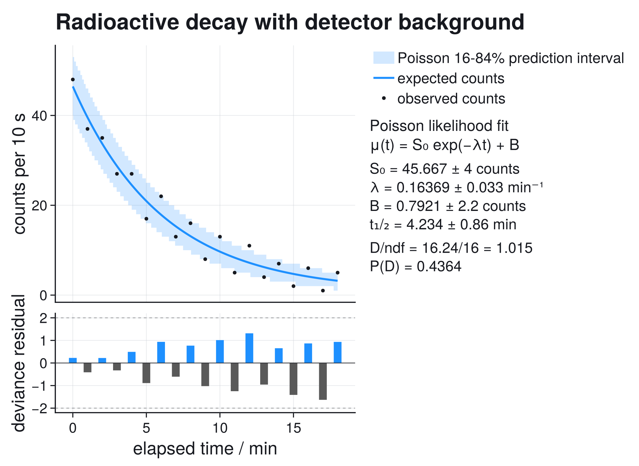
The observed points have no $\sqrt n$ error bars: near zero, such bars cannot represent the strongly asymmetric sampling distribution (Poisson Counts And Histograms). The shaded region instead spans the 16th to 84th percentiles of future Poisson counts predicted by the fitted model. It is a prediction interval for discrete observations, not a confidence band for the mean curve; it is conditional on the fitted mean and does not include parameter uncertainty. Because counts are discrete, its actual coverage changes in steps and is generally not exactly 68%.

The band edges are stepped: Poisson observations are integers, so the 16th and 84th percentiles can change only by whole counts as $\mu(t)$ varies, and the figure renders each change as a vertical edge instead of interpolating fractional count quantiles. The plateaus become wider at late times because the exponential mean approaches the background more slowly: $|\mathrm{d}\mu/\mathrm{d}t|$ decreases. The lower and upper edges jump at different times because the two percentiles cross different probability thresholds. The band is constructed from the fitted mean curve as quantile(Poisson(mu), 0.16) and quantile(Poisson(mu), 0.84) on a dense time grid; plot_fit draws Gaussian confidence and prediction bands only and does not produce this display.

Data

The count arrays are listed explicitly in the fit sections. They are controlled teaching records, not measurements attributed to a particular isotope or detector campaign; the listed integers are the complete input. The first series has a low-count tail; the second is an unequally binned pulse-height spectrum with one empty bin.

A one-bin sanity check: if the model predicts $\mu=0.7$ counts, observing $n=0$ is not pathological; it has probability $e^{-0.7}\approx0.50$. A Gaussian least-squares fit with $\sqrt n$ would assign zero uncertainty to the same observation.

Poisson Likelihood and Deviance

For independent counts,

\[n_i \sim \operatorname{Poisson}(\mu_i).\]

This statement assumes disjoint acquisition windows, independent events, known exposure and efficiency, and a stable background. Substantial dead time, pile-up, clustering, or an unmodelled exposure change breaks the model. If exposure differs between windows, that exposure belongs inside each $\mu_i$ rather than in an after-the-fact rescaling.

fit_poisson_model minimizes twice the negative log-likelihood:

\[C(p) = -2\log L(p) = 2\sum_i \left[ \mu_i(p)-n_i\log\mu_i(p)+\log\Gamma(n_i+1) \right].\]

The last term is the factorial, $\log\Gamma(n_i+1) = \log(n_i!)$. It depends only on the observed counts, not on $p$, so it never moves the minimum or changes the fitted parameters; it is kept so that $-2\log L$ stays on the absolute scale used for model comparison (Poisson Counts And Histograms).

The goodness-of-fit quantity is the Poisson deviance:

\[D = 2\sum_i \left[ \mu_i-n_i+n_i\log\!\left(\frac{n_i}{\mu_i}\right) \right],\]

where for $n_i = 0$ the bracket is exactly $\mu_i$ (the limit of $n_i\log(n_i/\mu_i)$ as $n_i \to 0$ is zero), so the term is $2\mu_i$; the same convention applies in the residual formula below. The lower plot shows signed deviance residuals,

\[r_i = \operatorname{sign}(n_i-\mu_i) \sqrt{ 2\left[ \mu_i-n_i+n_i\log\!\left(\frac{n_i}{\mu_i}\right) \right] }.\]

They put upward and downward count fluctuations on a roughly comparable scale. A structureless mix around zero supports the model; long runs with one sign, isolated large values, or dependence on the expected count level suggest a missing component or a wrong count model.

Complete Decay Fit

For count likelihoods, stats.chi2 stores the Poisson deviance, so stats.chi2_ndf is the deviance per degree of freedom and stats.pvalue (printed as P(D)) is its asymptotic chi-square p-value.

using ScientificFitting
using Printf

time_min = collect(0.0:1.0:18.0)
counts = [
    48, 37, 35, 27, 27, 17, 22, 13, 16, 8,
    13, 5, 11, 4, 7, 2, 6, 1, 5,
]

decay_model(t, p) = @. p[1] * exp(-p[2] * t) + p[3]

decay_result = fit_poisson_model(
    decay_model,
    time_min,
    counts;
    p0=[40.0, 0.15, 3.0],
    bounds=([1e-6, 1e-6, 1e-6], [200.0, 2.0, 50.0]),
    parameter_names=["initial signal", "decay constant", "background"],
    initial_guesses=[
        [70.0, 0.30, 2.0],
        [25.0, 0.08, 5.0],
    ],
)

lambda = decay_result.params[2]
sigma_lambda = decay_result.param_stderr[2]
half_life = log(2) / lambda
sigma_half_life = log(2) * sigma_lambda / lambda^2

@printf("half-life = %.3f +/- %.3f min\n", half_life, sigma_half_life)
@printf("background = %.3f +/- %.3f counts per 10 s\n",
        decay_result.params[3], decay_result.param_stderr[3])
@printf("deviance/ndf = %.3f\n", decay_result.stats.chi2_ndf)
@printf("P(D) = %.3f\n", decay_result.stats.pvalue)
println(diagnostic_dashboard_text(decay_result))

half-life = 4.234 +/- 0.863 min
background = 0.792 +/- 2.189 counts per 10 s
deviance/ndf = 1.015
P(D) = 0.436
Fit diagnostic dashboard
status = ok - no immediate issue
critical = 0, warning = 0, info = 0
No major diagnostic issues detected by the current checks.
No next action required by the current diagnostic checks.

Multiple initial guesses reduce the chance that one poor starting point defines the reported result for this nonlinear signal-plus-background model.

Interpretation: Decay Result

The result is approximately

\[\lambda = 0.164 \pm 0.033\ \mathrm{min}^{-1}, \qquad T_{1/2} = 4.23 \pm 0.86\ \mathrm{min}.\]

$\lambda$ and its error are decay_result.params[2] and decay_result.param_stderr[2]; the printed half-life and its error follow from them through the propagation lines in the code above.

The fitted background is $0.792\pm2.189$ counts per window in the local quadratic approximation. That symmetric interval extends below the physical positivity bound because the acquisition ends with only a few low-count windows, and should not be reported as the final background interval. A profile scan (Profiles And Contours) refits the signal parameters at each forced background value; if the profile does not reach the interval threshold before the background reaches zero, the lower interval edge is truncated by the physical bound: report an asymmetric interval or a one-sided upper limit. A longer background-only acquisition would separate source and detector background more directly.

The half-life uncertainty above is first-order propagation of the local $\lambda$ covariance. Transform a profile interval for $\lambda$ when the half-life uncertainty is central to the scientific conclusion.

The deviance is approximately $16.24$ for $16$ degrees of freedom (19 time windows minus 3 free parameters), giving an asymptotic p-value near $0.44$, compatible with the model (Goodness Of Fit).

Question Two: Where Is The Spectral Peak?

A pulse-height spectrum contains a Gaussian-like detector peak above a uniform background. The bins are unequal, including one empty low-amplitude bin: bin widths grow with amplitude, from 0.4 V at low amplitude to 1.8 V in the tail, so narrow bins resolve the onset of the spectrum while the sparse high-amplitude tail is not split into many near-empty bins. This is defensible only when the edges are fixed independently of the observed fluctuations and the model is integrated over those exact edges. The fitted quantities are peak yield $N$, centroid $m$, Gaussian width $s$, and background density $\rho_B$.

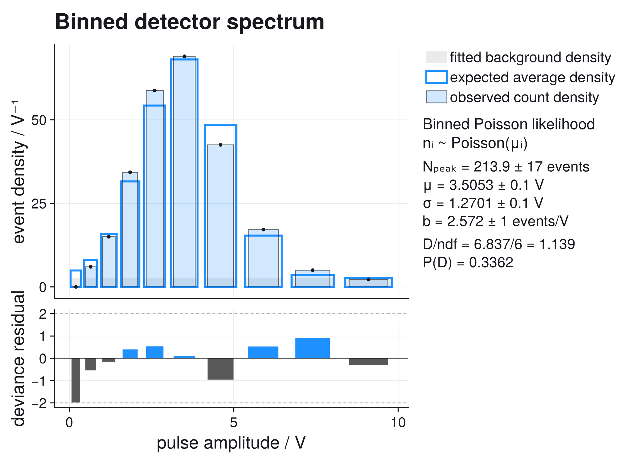
The model must return the expected count in each bin, not the density evaluated at the bin center. For bin edges $e_i$ and $e_{i+1}$,

\[\mu_i = N \left[ \Phi\!\left(\frac{e_{i+1}-m}{s}\right) - \Phi\!\left(\frac{e_i-m}{s}\right) \right] + \rho_B(e_{i+1}-e_i).\]

Here $\Phi$ is the standard normal cumulative distribution function (not the work function of the photoelectric-threshold example). The implementation expresses it through the error function, $\Phi(z) = \tfrac{1}{2}\left[1 + \operatorname{erf}(z/\sqrt{2})\right]$; in the difference $\Phi(a)-\Phi(b)$ the constant $\tfrac{1}{2}$ cancels, which yields the 0.5 * (erf(...) - erf(...)) factor in expected_counts below.

Evaluating the density only at bin centers can bias the peak position, width, and yield when bins differ in width or the density changes across a bin.

For display only, the upper panel divides observed and expected counts by each bin width: the bar height times the bin width equals the bin count (the observed bars are drawn slightly narrower than their bins for visual separation), and a uniform background appears flat instead of growing taller in wider bins. The likelihood and the lower-panel deviance residuals use the original integer counts.

Complete Histogram Fit

using ScientificFitting
using Printf
using SpecialFunctions

edges = [0.0, 0.4, 0.9, 1.5, 2.2, 3.0, 4.0, 5.2, 6.6, 8.2, 10.0]
counts = [0, 3, 9, 24, 47, 69, 51, 24, 8, 4]

function expected_counts(edges, p)
    peak_yield, centroid, width, background_density = p
    return [
        peak_yield * 0.5 * (
            erf((edges[i + 1] - centroid) / (sqrt(2) * width)) -
            erf((edges[i] - centroid) / (sqrt(2) * width))
        ) + background_density * (edges[i + 1] - edges[i])
        for i in 1:(length(edges) - 1)
    ]
end

spectrum_result = fit_histogram_model(
    expected_counts,
    edges,
    counts;
    p0=[210.0, 3.8, 1.0, 1.0],
    bounds=([1e-6, 0.0, 0.05, 1e-6], [1000.0, 10.0, 5.0, 100.0]),
    parameter_names=["peak yield", "centroid", "width", "background density"],
    initial_guesses=[
        [300.0, 4.2, 1.5, 0.5],
        [150.0, 3.2, 0.7, 2.0],
    ],
)

@printf("peak yield = %.1f +/- %.1f events\n",
        spectrum_result.params[1], spectrum_result.param_stderr[1])
@printf("centroid = %.3f +/- %.3f V\n",
        spectrum_result.params[2], spectrum_result.param_stderr[2])
@printf("width = %.3f +/- %.3f V\n",
        spectrum_result.params[3], spectrum_result.param_stderr[3])
@printf("background density = %.3f +/- %.3f events/V\n",
        spectrum_result.params[4], spectrum_result.param_stderr[4])
@printf("deviance/ndf = %.3f\n", spectrum_result.stats.chi2_ndf)
@printf("P(D) = %.3f\n", spectrum_result.stats.pvalue)
println(diagnostic_dashboard_text(spectrum_result))

peak yield = 213.9 +/- 17.3 events
centroid = 3.505 +/- 0.103 V
width = 1.270 +/- 0.100 V
background density = 2.572 +/- 1.035 events/V
deviance/ndf = 1.139
P(D) = 0.336
Fit diagnostic dashboard
status = ok - no immediate issue
critical = 0, warning = 0, info = 0
No major diagnostic issues detected by the current checks.
No next action required by the current diagnostic checks.

The fitted centroid and width are approximately

\[m = 3.505 \pm 0.103\ \mathrm{V}, \qquad s = 1.270 \pm 0.100\ \mathrm{V}.\]

The empty first bin remains informative: it penalizes models that predict too many low-amplitude events.

Diagnostics

The deviance is approximately $6.84$ for $6$ degrees of freedom (10 bins minus 4 free parameters), with an asymptotic p-value near $0.34$. A count model can have an acceptable global deviance while still missing structure in a narrow peak, a tail, or the empty bins, so inspect the deviance residual panel next: look for runs of same-sign residuals, one tail that is systematically high, or a peak that is too narrow.

The automatic dashboard reports ok because the optimizer converged, the covariance estimate is usable, and no generic fit pathology was detected; it does not prove that the Poisson process is the correct physical counting model.

What Can Go Wrong

The counts are background-subtracted. Differences of Poisson variables are not Poisson and can be negative. Fit source and background measurements jointly, or use a likelihood that represents the subtraction procedure.

The variance exceeds the mean. Dead time, pile-up, drift, clustering, or unmodelled rate changes can produce overdispersion. A Poisson likelihood then understates uncertainty even if the fitted curve looks plausible.

A bin is empty. Keep it. Empty bins constrain the expected rate and are handled naturally by the Poisson likelihood.

The result changes with binning. Check the expected-count integration, detector resolution model, and whether an unbinned or extended-unbinned likelihood is more appropriate.

The p-value is treated as exact. The chi-square approximation for the deviance is asymptotic. With very sparse counts, active bounds, or weakly identified parameters, calibrate goodness of fit by simulation before making a critical claim.

A parameter sits on its positivity bound. Local symmetric errors and asymptotic likelihood-ratio thresholds may be unreliable. Inspect a profile and report a one-sided limit when appropriate.

Next useful pages: Constraints and Profiles, Fitting for Practitioners, and Likelihoods and Model Comparison.