Quickstart
This page is the first complete ScientificFitting workflow. It is deliberately small, but it still follows the same logic as a real analysis:
- define the measured quantities and uncertainties,
- choose a model,
- fit,
- inspect the result,
- decide whether the result is trustworthy enough to use.
The data are synthetic, constructed for this tutorial: a straight line plus noise plus a deliberate smooth residual oscillation, so the first fit looks good and is still flagged for review. Complete analyses live in the Gallery.
Question
A sensor voltage $U$ should be approximately linear in an input position $x$. We want the calibration slope and offset, including uncertainties, and a plot that already shows whether the fit is plausible.
Data
We have three arrays:
x: measured input values,y: measured sensor output,sigma_y: one-standard-deviation uncertainty of each output value.
The uncertainties grow linearly from 0.16 V to 0.36 V across the range. Here they represent pointwise repeatability of the voltage reading after range-dependent noise has been characterized. A shared gain uncertainty would instead correlate points and should not be encoded as independent sigma_y values.
Model
The first model is a straight line:
\[U(x) = m x + b.\]
For independent Gaussian y uncertainties, ScientificFitting minimizes
\[\chi^2(m,b) = \sum_i \left( \frac{U_i-(m x_i+b)}{\sigma_{U,i}} \right)^2.\]
The sum runs over all data points; $U_i$ is the measured output y[i] at position $x_i$, and $\sigma_{U,i}$ is its standard deviation sigma_y[i].
This is the standard weighted least-squares model. It is appropriate only if the uncertainties are meaningful standard deviations and the residuals are roughly Gaussian and structureless.
Complete Code
Running this block requires both ScientificFitting and CairoMakie in the active environment (see Installation). In a repository checkout, use the docs environment, which provides both: julia --project=docs.
using ScientificFitting
using CairoMakie

# Measured calibration points. sigma_y is the one-standard-deviation
# uncertainty of each voltage reading.
x = [0.0, 0.4348, 0.8696, 1.3043, 1.7391, 2.1739, 2.6087, 3.0435,
     3.4783, 3.9130, 4.3478, 4.7826, 5.2174, 5.6522, 6.0870, 6.5217,
     6.9565, 7.3913, 7.8261, 8.2609, 8.6957, 9.1304, 9.5652, 10.0]
y = [0.7000, 1.6125, 2.4832, 3.2749, 3.9858, 4.6545, 5.3439, 6.1123,
     6.9838, 7.9338, 8.8975, 9.7983, 10.5849, 11.2581, 11.8738,
     12.5193, 13.2732, 14.1663, 15.1641, 16.1797, 17.1125, 17.8965,
     18.5336, 19.0964]
sigma_y = [0.1600, 0.1687, 0.1774, 0.1861, 0.1948, 0.2035, 0.2122,
           0.2209, 0.2296, 0.2383, 0.2470, 0.2557, 0.2643, 0.2730,
           0.2817, 0.2904, 0.2991, 0.3078, 0.3165, 0.3252, 0.3339,
           0.3426, 0.3513, 0.3600]

fit = fitplot(
    x,
    y;
    sigma_y=sigma_y,
    title="Quickstart calibration",
    model_label="U(x) = m x + b",
    xlabel="x",
    xunit="mm",
    ylabel="U",
    yunit="V",
    parameter_names=["m", "b"],
    band=:prediction,
    nsigma=1,
    band_label="1σ prediction band",
    show_legend=true,
    show_panel=true,
    print_report=true,
    filename="quickstart_linear.pdf",
)

result = fit.result

println()
println(diagnostic_dashboard_text(result))Fit report backend = lsqfit converged = true iterations = unavailable message = Converged with LsqFit Parameters: m = 1.847 +/- 0.017 b = 0.737 +/- 0.077 Statistics: cost = chi2 cost_min = 11.0224 minus2loglik_min = -10.881 chi2 = 11.0224 ndf = 22 chi2/ndf = 0.501018 pvalue = 0.974428 AIC = -6.88096 BIC = -4.52485 Fit diagnostic dashboard status = review - inspect diagnostics critical = 0, warning = 2, info = 0 2 warning(s). Inspect before trusting uncertainties or conclusions. Next actions: 1. Use a covariance model, inspect acquisition order/time dependence, or fit a model with the missing systematic component. 2. Look for missing model structure, drift, a calibration offset, or correlated uncertainty in that interval.
The report header records which numerical solver ran (backend, chosen automatically or via the solver keyword), whether it reported convergence, and its status message; LsqFit reports no iteration count, hence iterations = unavailable. cost names the minimized objective — here the chi-square — and cost_min is its value at the minimum.
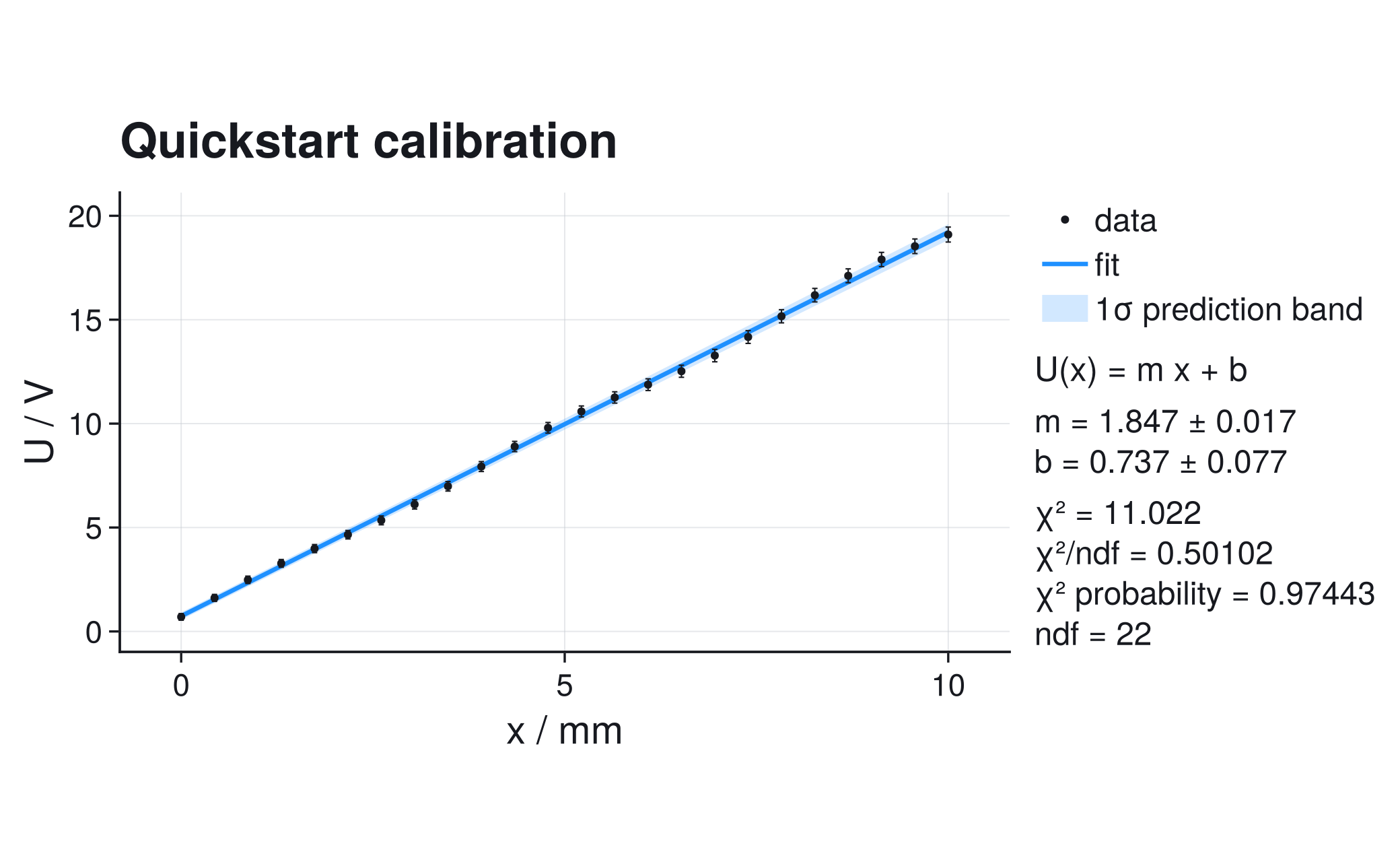
show_panel=true puts the numerical summary beside the axes; print_report=true prints the full text report to the terminal; the panel shows a compact subset of it. nsigma sets the band half-width in standard deviations; band_label is free text and should be kept consistent with it. filename additionally saves the figure to that file in the working directory. The returned fit.figure is an ordinary Makie figure.
fitplot(x, y; sigma_y=...) uses a straight-line model by default. If you want to make the model explicit, use:
model(x, p) = @. p[1] * x + p[2]
result = fit_model(model, x, y; p0=[1.0, 0.0], sigma_y=sigma_y)
p0 is the vector of starting parameter values for the iterative optimizer; its order defines how the model reads them (p[1] = slope, p[2] = intercept here), and every explicit model call requires it. A rough estimate read off the data is sufficient for well-behaved models; for nonlinear models a poor start can make the optimizer fail or converge to a wrong local minimum. The line-only fitplot(x, y; ...) call above needed no p0 because it derives start values from the first and last data points.
The explicit form is preferred once the model is not a straight line.
What The Plot Means
The theme keyword of fitplot (default :sans) changes only typography and visual hierarchy, never the data, fit, band, or reported numbers. The plot contains:
- measured data points,
- y error bars from
sigma_y, - the fitted line,
- a 1σ prediction band,
- a report panel with fitted parameters and fit statistics.
A prediction band is wider than a confidence band for the mean curve. It asks: where would a new measurement plausibly land, given the fitted model and the measurement uncertainty?
If you want only the uncertainty of the fitted mean curve, use band=:confidence.
Interpreting The Result
The fitted calibration coefficients are
\[m = (1.847 \pm 0.017)\,\mathrm{V\,mm^{-1}}, \qquad b = (0.737 \pm 0.077)\,\mathrm{V}.\]
These are local one-standard-deviation errors from the parameter covariance: "local" means derived from the curvature of the cost function at the minimum, reliable only when the cost is approximately parabolic there (see profiles when it is not). They describe the stated independent-Gaussian model; they do not include an unmodelled shared calibration uncertainty or residual correlation.
The most important fields are:
result.params: best-fit parameter values.result.param_stderr: local one-standard-deviation parameter errors.result.param_covariance: local parameter covariance matrix.result.stats.chi2: weighted residual sum of squares.result.stats.chi2_ndf: chi-square divided by the degrees of freedom, the number of data points minus the number of free parameters (here 24 − 2 = 22; see Degrees Of Freedom).result.stats.pvalue: the probability of a chi-square at least as large as the observed one if the model and the uncertainties are correct; see Goodness Of Fit.
As a rule of thumb, $\chi^2/\mathrm{ndf}$ should be near one when the model and uncertainties are both plausible. Much larger values usually mean missing model structure, underestimated uncertainties, outliers, or wrong correlations. Much smaller values can mean overestimated uncertainties or non-independent data.
Here $\chi^2/\mathrm{ndf}=0.50$ and $p=0.974$ are not evidence of an exceptionally accurate calibration. Together with the smooth residual pattern, they suggest that the pointwise errors are conservative, correlated, or both. The numerical coefficients are useful for continuing the analysis, but the uncertainty model needs review before they become a final calibration result.
The report also exposes normalized likelihood and information-criterion fields for later model comparisons. minus2loglik_min includes the Gaussian normalization and may be negative; its absolute value is not a goodness-of-fit score. AIC and BIC likewise have no useful absolute target. Compare them only between candidate models fitted to the same observations with the same likelihood definition.
First Diagnosis
The dashboard summarizes the first things to inspect:
dashboard = diagnostic_dashboard(result)diagnostic_dashboard(result) returns the dashboard as a structured object; diagnostic_dashboard_text(result), used in the Complete Code block above, renders the same dashboard as text. Its status line uses three labels:
ok - no immediate issue: no major issue found by the current checks,review - inspect diagnostics: warnings exist; inspect before using the result,critical - fix before use: at least one critical issue exists and must be fixed before the result is used for conclusions.
For this synthetic example, review - inspect diagnostics follows from the low chi-square and from the smooth residual pattern. Both warnings point to the same inspection: check the residuals in acquisition order and replace the independent-error model if a shared or time-correlated component is physically justified.
The dashboard does not prove the model is true. It only catches common failure modes quickly: bad goodness-of-fit, active bounds, ill-conditioned covariance, large pulls, structured residuals, strong parameter correlations, and failed optimizer convergence.
What Can Go Wrong
A straight-line calibration can look visually acceptable and still be wrong. Inspect the fit more carefully if:
- residuals curve systematically above and below the line,
- the prediction band is much narrower than the observed scatter,
- $\chi^2/\mathrm{ndf}$ is far from one,
- the p-value is extremely small or extremely close to one,
- parameters are strongly correlated,
- one or two points dominate the result.
If the model is nonlinear, bounded, or weakly constrained, local symmetric errors may be misleading. Use profile intervals and contours:
prof = profile(result, 1; adaptive=true)
interval = profile_interval(result, 1)
cont = ScientificFitting.contour(result, 1, 2; adaptive=true)
The integer arguments are parameter indices in the fitted parameter vector (1 = m, 2 = b here). adaptive=true refines the scan near the points where the profile crosses the interval threshold instead of forcing a dense grid. ScientificFitting.contour is written qualified because Makie exports a contour of its own. Profiles and contours explains how to read the results.
Next Steps
- Fitting for Practitioners for practical troubleshooting rules.
- How ScientificFitting Works for the object flow behind the one-line interface.
- Gaussian least squares for the derivation of weighted chi-square, and profiles when a local symmetric error is not enough.