Photoelectric Work Function
This workflow estimates the work function of a metal from photoelectric stopping-voltage measurements. The baseline and emission regimes are fitted separately; the threshold is the intersection of the two fitted lines, with uncertainty propagated from both covariance matrices.
Question
Light with frequency $\nu$ ejects electrons only if the photon energy exceeds the material work function $\Phi$. After subtracting the instrument baseline, the stopping-voltage excess measures the maximum kinetic energy:
\[e\,[U_\mathrm{emit}(\nu)-U_\mathrm{base}(\nu)] = h(\nu-\nu_0), \qquad \nu \ge \nu_0, \qquad \Phi=h\nu_0.\]
The analysis extracts the Planck constant $h$ from the slope, the work function $\Phi$ from the threshold energy, and the threshold frequency $\nu_0$ where emission starts.
Data
This is a controlled teaching dataset, not archival experimental data. The columns are frequency, stopping voltage, and individual standard uncertainties in both quantities: eight points resolve the baseline below the transition, ten the emission regime. The uncertainties differ from point to point (heteroskedastic) because frequency calibration and voltage readout precision change across the scan.
Below the threshold no photoelectrons are emitted, so no stopping voltage exists there in the strict sense; the voltage recorded in that regime is the zero-current readout of the measurement chain (offset and drift). That is why those eight points enter the fit as an instrument baseline instead of being forced to zero.
The regime assignment is an experimental decision made before the fit, not an opportunistic choice of whichever line a transition-region point happens to favor.
Model
Both regimes are locally linear and parameterized around $\nu_\mathrm{ref}=550\,\mathrm{THz}$, close to the transition, rather than around the physically irrelevant $\nu=0$:
\[U_\mathrm{base}(\nu) = m_\mathrm{base}(\nu-\nu_\mathrm{ref}) + c_\mathrm{base}, \qquad U_\mathrm{emit}(\nu) = m_\mathrm{emit}(\nu-\nu_\mathrm{ref}) + c_\mathrm{emit}.\]
Centering does not change either line; it reduces the artificial slope-intercept correlation and makes $c$ the fitted voltage near the threshold region.
The baseline slope belongs to the readout chain, not to the photoelectric effect. The physical slope is the difference
\[m_\gamma=m_\mathrm{emit}-m_\mathrm{base} = \frac{10^{12}h}{e},\]
when frequency is measured in THz. The threshold offset and absolute frequency are
\[x_0 = \frac{c_\mathrm{base}-c_\mathrm{emit}}{m_\gamma}, \qquad \nu_0=\nu_\mathrm{ref}+x_0.\]
The denominator is the difference of two fitted slopes, so nearly parallel lines would let the same voltage noise move the intersection by a large amount; the covariance matrices of both fitted lines are propagated through this formula.
The work function follows from the threshold photon energy: since $\Phi = h\nu_0$ and $h = 10^{-12}\,e\,m_\gamma$, the factors of $e$ and $10^{12}$ cancel when $\Phi$ is expressed in eV and $\nu_0$ in THz:
\[\Phi[\mathrm{eV}] = m_\gamma[\mathrm{V/THz}]\, \nu_0[\mathrm{THz}].\]
Fit
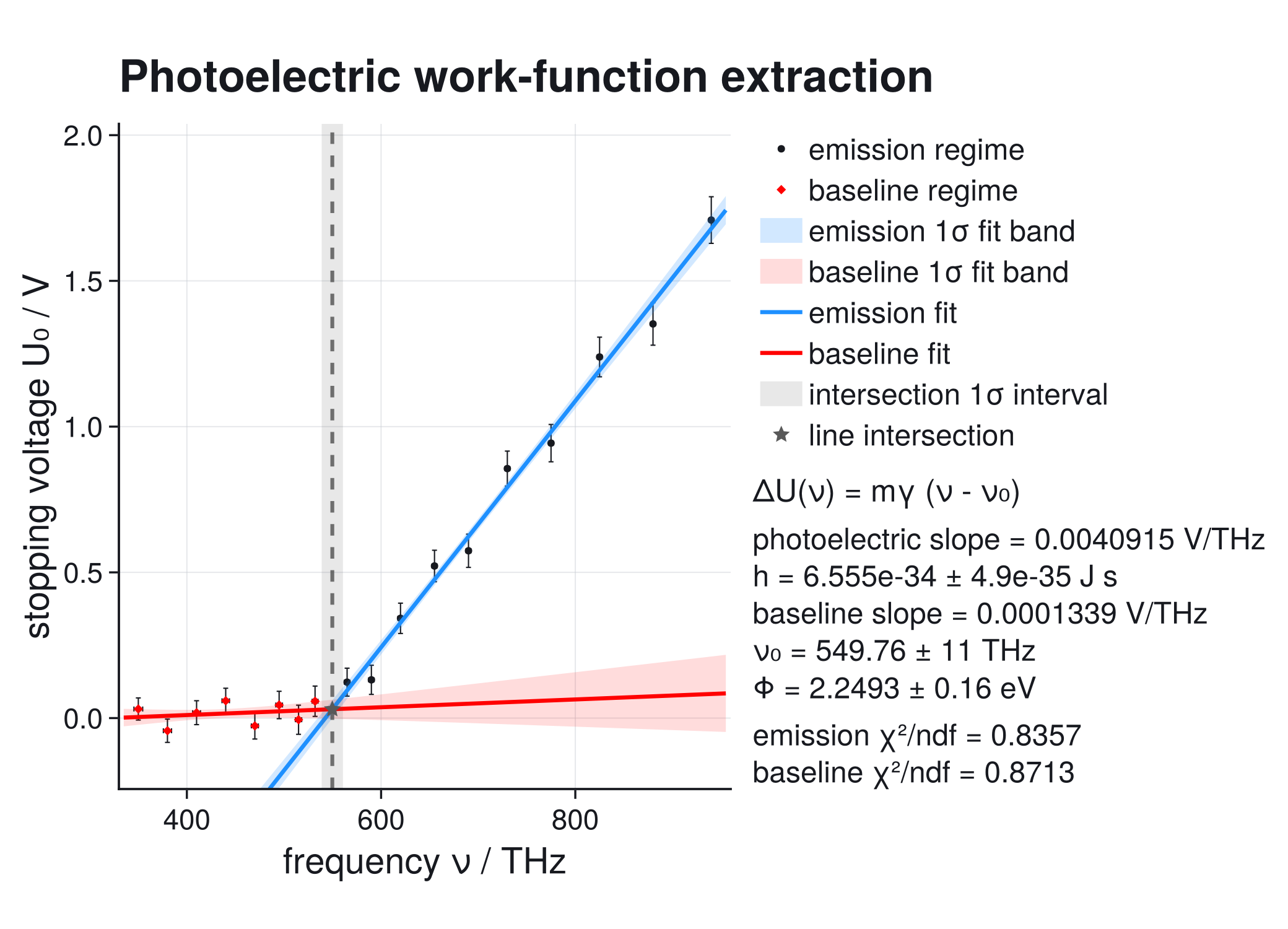
The plot in the Plot Construction section below is constructed from the same two FitResults; no refit occurs during rendering.
The start values come from the physics: for a nearly flat baseline the expected emission slope is $10^{12}h/e \approx 4.1\times10^{-3}\,\mathrm{V/THz}$, so p0 starts the emission slope at 0.0042; the baseline starts at zero slope for the same reason. No bounds are set — the fit reaches the same minimum even from a flat-slope start, and a fit that ends on an active bound would make the local covariance unreliable (see Fixed Parameters And Bounds).
using ScientificFitting
using LinearAlgebra
using Printf

const elementary_charge = 1.602176634e-19

frequency_THz = [350.0, 380.0, 410.0, 440.0, 470.0, 495.0, 515.0, 532.0,
                 565.0, 590.0, 620.0, 655.0, 690.0, 730.0, 775.0, 825.0,
                 880.0, 940.0]
voltage_V = [0.0312, -0.0434, 0.01855, 0.0594, -0.02685, 0.04495, -0.0057,
             0.05784, 0.12324, 0.13123, 0.34230, 0.52185, 0.57404, 0.85602,
             0.94333, 1.23891, 1.35237, 1.70871]
sigma_frequency_THz = [4.5, 4.2, 4.0, 3.8, 3.6, 3.4, 3.2, 3.0,
                       2.9, 2.8, 2.7, 2.6, 2.5, 2.5, 2.4, 2.4, 2.3, 2.3]
sigma_voltage_V = [0.038, 0.040, 0.041, 0.043, 0.045, 0.047, 0.050, 0.052,
                   0.048, 0.050, 0.052, 0.054, 0.057, 0.060, 0.064, 0.068,
                   0.073, 0.080]

baseline_mask = frequency_THz .<= 532.0
emission_mask = .!baseline_mask
reference_frequency_THz = 550.0
line_model(nu_THz, p) = @. p[1] * (nu_THz - reference_frequency_THz) + p[2]

baseline = fit_model(
    line_model,
    frequency_THz[baseline_mask],
    voltage_V[baseline_mask];
    p0=[0.0, 0.02],
    sigma_y=sigma_voltage_V[baseline_mask],
    sigma_x=sigma_frequency_THz[baseline_mask],
)

emission = fit_model(
    line_model,
    frequency_THz[emission_mask],
    voltage_V[emission_mask];
    p0=[0.0042, 0.02],
    sigma_y=sigma_voltage_V[emission_mask],
    sigma_x=sigma_frequency_THz[emission_mask],
)

me, ce = emission.params
mb, cb = baseline.params
photoelectric_slope = me - mb
threshold_offset_THz = (cb - ce) / photoelectric_slope
threshold_THz = reference_frequency_THz + threshold_offset_THz

gradient_emission = [
    -threshold_offset_THz / photoelectric_slope,
    -1 / photoelectric_slope,
]
gradient_baseline = [
    threshold_offset_THz / photoelectric_slope,
    1 / photoelectric_slope,
]
threshold_variance =
    dot(gradient_emission, emission.param_covariance * gradient_emission) +
    dot(gradient_baseline, baseline.param_covariance * gradient_baseline)
sigma_threshold_THz = sqrt(threshold_variance)

h_fit = photoelectric_slope * elementary_charge / 1e12
sigma_photoelectric_slope = sqrt(
    emission.param_covariance[1, 1] + baseline.param_covariance[1, 1],
)
sigma_h = sigma_photoelectric_slope * elementary_charge / 1e12

work_function_eV = photoelectric_slope * threshold_THz
work_gradient_emission = [reference_frequency_THz, -1.0]
work_gradient_baseline = [-reference_frequency_THz, 1.0]
work_variance =
    dot(work_gradient_emission,
        emission.param_covariance * work_gradient_emission) +
    dot(work_gradient_baseline,
        baseline.param_covariance * work_gradient_baseline)
sigma_work_function_eV = sqrt(work_variance)

@printf("h = %.5e +/- %.5e J s\n", h_fit, sigma_h)
@printf("Phi = %.4f +/- %.4f eV\n", work_function_eV, sigma_work_function_eV)
@printf("nu0 = %.3f +/- %.3f THz\n", threshold_THz, sigma_threshold_THz)
println()
println("baseline")
println(diagnostic_dashboard_text(baseline))
println("emission")
println(diagnostic_dashboard_text(emission))h = 6.55527e-34 +/- 4.89176e-35 J s Phi = 2.2493 +/- 0.1635 eV nu0 = 549.759 +/- 10.954 THz baseline Fit diagnostic dashboard status = ok - no immediate issue critical = 0, warning = 0, info = 0 No major diagnostic issues detected by the current checks. No next action required by the current diagnostic checks. emission Fit diagnostic dashboard status = review - inspect diagnostics critical = 0, warning = 1, info = 0 1 warning(s). Inspect before trusting uncertainties or conclusions. Next actions: 1. Use a covariance model, inspect acquisition order/time dependence, or fit a model with the missing systematic component.
The baseline dashboard is quiet; the emission fit draws one residual-correlation warning, whose named next check is the residuals in acquisition order. Neither status changes the propagation: parameter covariances are retained in full when computing $\nu_0$ and $\Phi$, and a quiet dashboard would not justify dropping slope-intercept correlation either.
The warning names its own check: plot the pulls in acquisition order. Doing that here shows no trend, no drift, and no cluster of same-sign residuals; the flag comes from the lag-1 autocorrelation of the pulls, which is negative — neighboring residuals alternate in sign slightly more often than chance predicts, just past the 2σ threshold of that check. A drift or a missing systematic would produce the opposite signature, positive autocorrelation with runs of same-sign residuals, so the suggested fixes do not apply. With ten points, one check slightly past its threshold is accepted as a false alarm, and the propagated uncertainties are quoted as they stand. With real data, repeat this inspection against the acquisition log before quoting them.
Interpretation
The fitted quantities are
\[h=(6.56\pm0.49)\times10^{-34}\,\mathrm{J\,s}, \qquad \nu_0=(549.8\pm11.0)\,\mathrm{THz},\]
and
\[\Phi=(2.25\pm0.16)\,\mathrm{eV}.\]
The fitted $h$ differs from the exact SI value $6.62607015\times10^{-34}\,\mathrm{J\,s}$ by about $0.15\sigma$. For controlled teaching data this agreement checks the analysis and uncertainty propagation, not the SI constant or a particular photocathode material.
Plot Construction
The numerical work is already in baseline, emission, and the propagated intersection quantities; the figure layers experiment-specific Makie annotations on top of ScientificFitting's plot theme, palette, and information panel. This is the intended lab-notebook pattern: fit once, keep the FitResults, then add annotations such as the threshold, an accepted region, or a literature line.
using CairoMakie
using ScientificFitting

style = :sans
appearance = :light
palette = plot_palette(style; appearance=appearance)
baseline_color = palette.secondary_color
threshold_color = palette.reference_color

fig = with_theme(plot_theme(style; appearance=appearance)) do
    Figure(size=(1120, 700))
end

ax = Axis(fig[1, 1];
    title="Photoelectric threshold from two fitted regimes",
    xlabel="frequency ν / THz",
    ylabel="stopping voltage U₀ / V")

errorbars!(ax, frequency_THz, voltage_V, sigma_voltage_V;
           color=palette.yerr_color,
           whiskerwidth=palette.error_whiskerwidth)
errorbars!(ax, frequency_THz, voltage_V, sigma_frequency_THz;
           direction=:x,
           color=palette.xerr_color,
           whiskerwidth=palette.error_whiskerwidth)
scatter!(ax, frequency_THz[baseline_mask], voltage_V[baseline_mask];
         color=baseline_color, marker=:diamond, label="baseline")
scatter!(ax, frequency_THz[emission_mask], voltage_V[emission_mask];
         color=palette.data_color, label="emission")

xgrid = collect(range(minimum(frequency_THz) - 15,
                      maximum(frequency_THz) + 15; length=500))
J = hcat(xgrid .- reference_frequency_THz, ones(length(xgrid)))

for (result, color, label) in (
    (baseline, baseline_color, "baseline fit"),
    (emission, palette.fit_color, "emission fit"),
)
    ygrid = line_model(xgrid, result.params)
    variance = vec(sum((J * result.param_covariance) .* J; dims=2))
    sigma_fit = sqrt.(clamp.(variance, 0.0, Inf))
    band!(ax, xgrid, ygrid .- sigma_fit, ygrid .+ sigma_fit;
          color=(color, 0.22), label="$label 1σ")
    lines!(ax, xgrid, ygrid;
           color=color, linewidth=palette.fit_linewidth, label=label)
end

add_vband!(ax,
           threshold_THz - sigma_threshold_THz,
           threshold_THz + sigma_threshold_THz;
           color=(threshold_color, 0.14),
           label="threshold 1σ")
add_vline!(ax, threshold_THz;
           color=threshold_color, linestyle=:dash, linewidth=2)
intersection_voltage = line_model([threshold_THz], emission.params)[1]
add_points!(ax, [threshold_THz], [intersection_voltage];
            marker=:star5, markersize=18, color=threshold_color,
            label="line intersection")

plot_info_panel!(
    fig[1, 2];
    legend_source=ax,
    model_label="ΔU(ν) = mγ (ν - ν₀)",
    parameter_lines=[
        "photoelectric slope = $(round(photoelectric_slope; sigdigits=5)) V/THz",
        "h = $(round(h_fit; sigdigits=4)) ± $(round(sigma_h; sigdigits=2)) J s",
        "baseline slope = $(round(mb; sigdigits=4)) V/THz",
        "ν0 = $(round(threshold_THz; sigdigits=5)) ± $(round(sigma_threshold_THz; sigdigits=2)) THz",
        "Φ = $(round(work_function_eV; sigdigits=5)) ± $(round(sigma_work_function_eV; sigdigits=2)) eV",
    ],
    statistic_lines=[
        "emission χ²/ndf = $(round(emission.stats.chi2_ndf; sigdigits=4))",
        "baseline χ²/ndf = $(round(baseline.stats.chi2_ndf; sigdigits=4))",
    ],
    theme=style,
    appearance=appearance,
)

save("photoelectric_threshold.pdf", fig)
All colors, error bars, line widths, and report typography come from the selected plot style; style=:tex or appearance=:dark restyles the whole figure coherently.
Error Propagation
Each fit returns a local covariance matrix for its slope and intercept. With independent measurements in the two regimes, the joint covariance is block diagonal:
\[V_\mathrm{joint} = \begin{pmatrix} V_\mathrm{emit} & 0 \\ 0 & V_\mathrm{base} \end{pmatrix}.\]
For $D=m_\gamma$ and $x_0=\nu_0-\nu_\mathrm{ref}$, differentiating $\nu_0=\nu_\mathrm{ref}+(c_\mathrm{base}-c_\mathrm{emit})/D$ with respect to each of the four line parameters, with $\partial D/\partial m_\mathrm{emit}=1$ and $\partial D/\partial m_\mathrm{base}=-1$, gives the threshold gradients with respect to the centered line parameters $(m,c)$:
\[\nabla_\mathrm{emit}\nu_0 = \begin{pmatrix}-x_0/D & -1/D\end{pmatrix}, \qquad \nabla_\mathrm{base}\nu_0 = \begin{pmatrix}x_0/D & 1/D\end{pmatrix}.\]
The propagated threshold variance is:
\[\sigma_{\nu_0}^2 = (\nabla_\mathrm{emit}\nu_0) V_\mathrm{emit} (\nabla_\mathrm{emit}\nu_0)^T + (\nabla_\mathrm{base}\nu_0) V_\mathrm{base} (\nabla_\mathrm{base}\nu_0)^T.\]
This includes the slope-intercept correlation within both lines; if the regimes share calibration systematics, the zero off-diagonal blocks are invalid and the shared terms must be included explicitly.
The other two propagated quantities use
\[h = \frac{eD}{10^{12}}, \qquad \Phi = D\nu_0 = D\nu_\mathrm{ref}+c_\mathrm{base}-c_\mathrm{emit}.\]
The second form for $\Phi$ makes its gradient transparent and shows why $m_\mathrm{emit}\nu_0$ would be wrong when the fitted baseline has a nonzero slope.
Reading The Plot
The vertical shaded interval is the propagated 1σ uncertainty of the line intersection — not the width of the physical transition and not a prediction interval for future observations. The shaded band along each fitted line is the 1σ uncertainty of the fitted mean line, propagated from the parameter covariance; it excludes new-observation noise and is narrower than a prediction band. Horizontal and vertical error bars show the individual measurement uncertainties.
Diagnostics
First checks for this workflow:
- $\chi^2/\mathrm{ndf}$ should be of order one if the linear model and uncertainties are realistic (Goodness Of Fit); the info panel in the figure reports 0.8713 for the baseline fit and 0.8357 for the emission fit.
- Residuals within either regime should not bend systematically; curvature would signal contact potentials, wavelength calibration errors, or a bad threshold selection.
- The fitted threshold should lie between the last baseline and the first emission measurement.
- A profile scan of the slope or intercept is useful when the threshold region is sparse, because local covariance can look too confident near a kink or bound.
If a diagnostic dashboard reports a review or critical status, check the model range, uncertainty model, and profile intervals before styling the plot.
What Can Go Wrong
Do not force the below-threshold baseline to exactly zero unless the measurement chain guarantees it; a fitted baseline accounts for offset and drift, and its uncertainty contributes to the threshold uncertainty.
Do not calculate the intersection from best-fit values and then forget the covariances; the threshold depends on all four line parameters.
If the residuals curve, the p-value is implausibly small, or the profile is non-parabolic, the local symmetric errors are not enough evidence for a careful scientific report.
Next useful pages: XY Uncertainties, Constraints and Profiles, and External Parameter Information.