Plotting And Customization
ScientificFitting's plotting layer is an optional CairoMakie extension: fitting, reporting, diagnostics, profiles, and contours work without Makie; loading CairoMakie adds the visual interface. A plot reads an existing fit result and never changes the numerical analysis.
The Short Path
fitplot combines fitting and plotting for notebook work:
using ScientificFitting
using CairoMakie

out = fitplot(
    model,
    x,
    y;
    p0=[1.0, 0.0],
    sigma_y=sigma_y,
    xlabel="position",
    xunit="mm",
    ylabel="voltage",
    yunit="V",
    show_panel=true,
)

result = out.result
fig = out.figure
All fitplot methods return the named tuple (result, figure).
When an x-y FitResult already exists, plot_fit(result) returns a Makie Figure without rerunning the optimizer:
fig = plot_fit(result; title="Sensor calibration")Reusable Styles
FitPlotStyle collects the visual tokens shared by every plot function. Each field overrides the corresponding token of the selected theme preset; nothing keeps the theme value. One style object works for plot_fit, fitplot, and all diagnostic plot functions via their style keyword. Content and layout choices (labels, panels, legends) remain per-function keywords; Makie-level details go through the *_kwargs arguments below.
The tokens are figure_size, panel_gap, data_color, data_marker, data_markersize, data_strokecolor, data_strokewidth, fit_color, fit_linewidth, band_color, band_alpha, xerr_color, yerr_color, error_linewidth, error_whiskerwidth, secondary_color, reference_color, stats_fontsize, stats_box_color, stats_box_alpha, stats_box_strokecolor, and stats_box_strokewidth.
project_style = FitPlotStyle(
    fit_color=:firebrick,
    band_alpha=0.25,
    data_markersize=7.0,
)

fig = plot_fit(result; style=project_style)
res_fig = plot_residuals(result; style=project_style)
Reports, Legends, And Panels
Report, panel, and legend are independent switches:
show_panel=trueincludes the numerical result panel in the figure;print_report=trueprintsreport_text(result)to the terminal;show_legend=truecontrols the legend independently.
Both fitplot and plot_fit default to show_panel=true; only fitplot has print_report, since plot_fit never prints.
plot_fit(
    result;
    show_panel=true,
    stats_position=:right,   # or :inside
    show_legend=true,
    stats_mode=:compact,     # or :full
)
With stats_position=:right, the legend sits above the parameter summary in the same left-aligned panel; with stats_position=:inside, legend_position and inside_stats_position set the in-axis locations. show_panel=false removes the panel.
The :sans theme preset (the default; see Two Visual Styles below) uses a (1040, 640) logical-pixel canvas with a right-side panel and (860, 560) without one; :tex uses (1000, 640) and (760, 520). style=FitPlotStyle(figure_size=(width, height)) requests a minimum logical canvas: a request too small for the measured legends, labels, and panel content grows rather than clips, and extra width goes to the flexible data axis once the panel has its natural width.
stats_panel_width=:auto uses that natural width; a value above 1 sets the preferred wrapping width in logical pixels, and a value in (0, 1] is a fraction of the figure width, clamped to 300–560 px. Legends and unbreakable TeX expressions may widen the panel.
Two Visual Styles
A theme describes visual properties only; it never changes data, fit, uncertainty band, statistics, or whether a panel is present. Warning labels on diagnostic figures are controlled separately through the diagnostic plot functions' panel_status_mode keyword (:issues, :all, or :none; see the diagnostics API).
theme=:sansis the default: sans-serif type, neutral filled observations, a saturated blue fit, visible grid guides, open axes (no top or right frame line), and a left-aligned title.theme=:texdiffers from:sansonly in the following: TeX typography, a full axis frame with inward ticks and no grid, hollow observations, and the blue/vermillion pair from the Okabe-Ito palette (designed to stay distinguishable in print and for color-vision deficiency) when multiple curves require color.
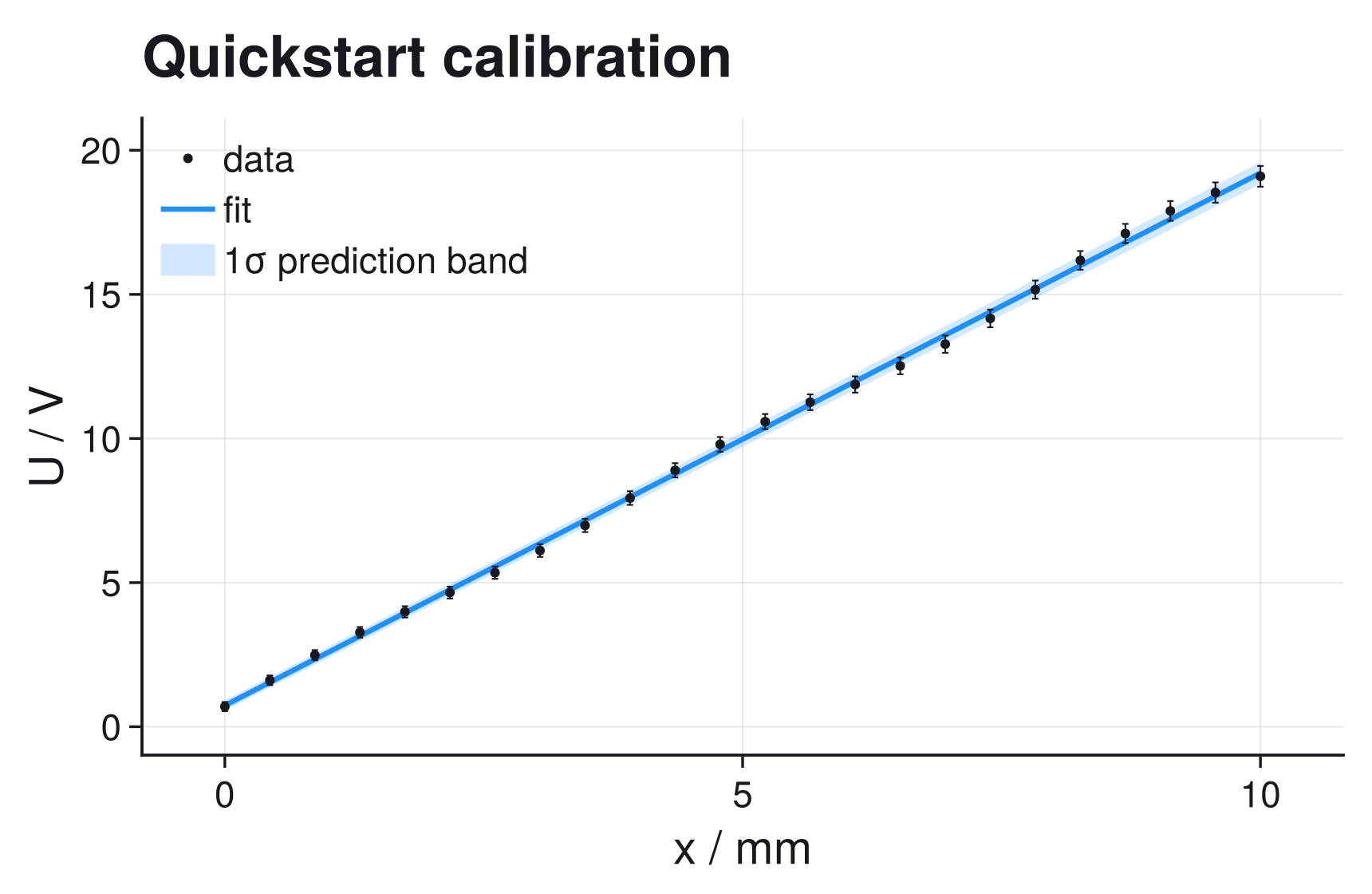
sans
Sans-serif typography, open axes, filled observations, and light grid guides.
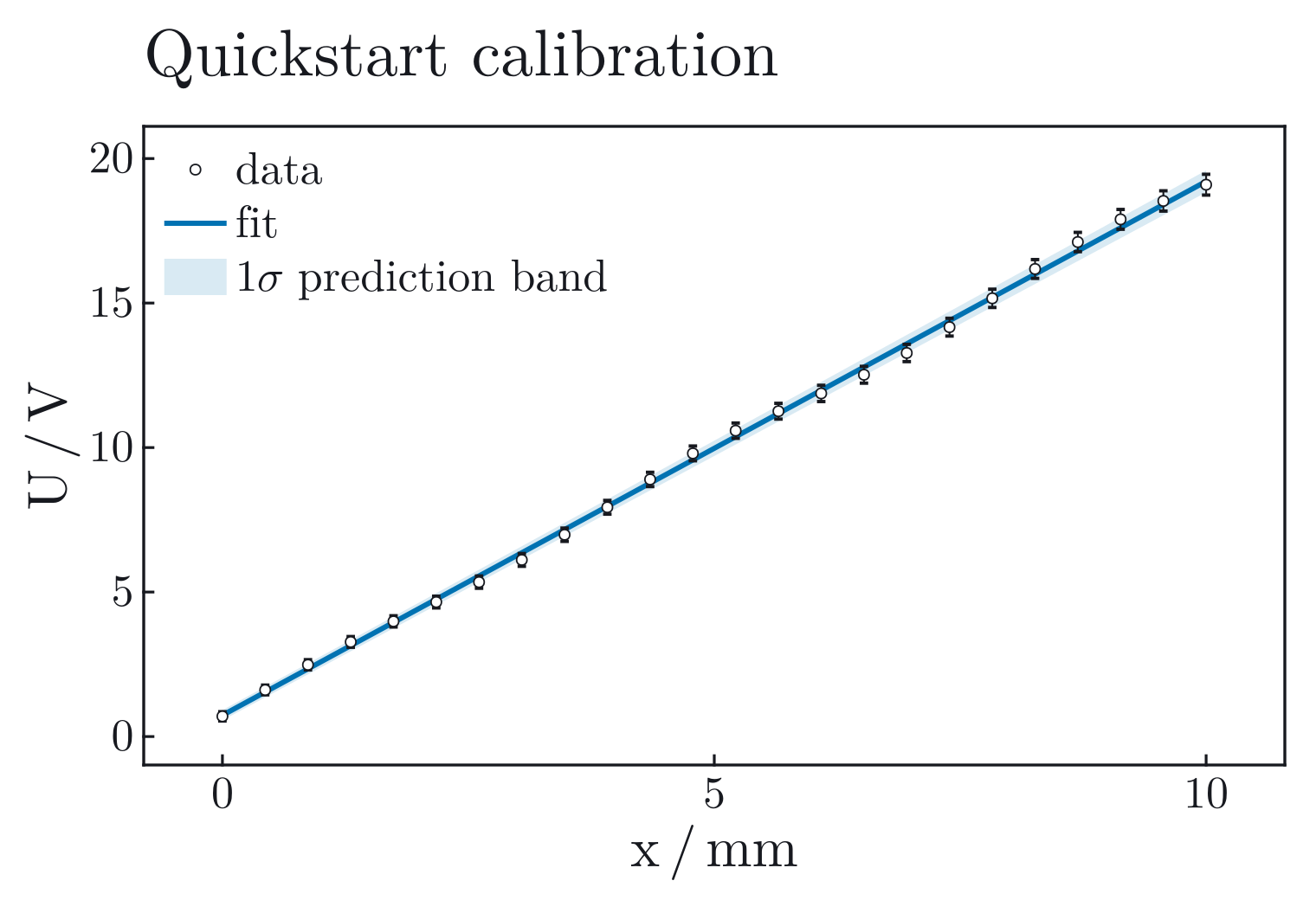
tex
TeX typography, a full frame, inward ticks, hollow observations, and no grid.
Color appearance is independent of style:
plot_fit(result; theme=:sans, appearance=:dark)appearance=:auto currently resolves to the light appearance; select :light or :dark explicitly when an exported asset must match a document.
LaTeX conversion is also independent:
using LaTeXStrings

plot_fit(
    result;
    theme=:tex,
    latex_labels=true,
    latex_stats=true,
    model_label=L"U_0(\nu)=h\nu/e-\Phi/e",
    xlabel=L"\nu",
    xunit=L"\mathrm{THz}",
)
Under TeX typography alone (latex_labels=false), plain strings are passed through unchanged. With latex_labels=true, a plain string containing \, ^, or _ is interpreted as TeX math; other strings render as upright text. Pass a LaTeXString, such as L"\nu", whenever a label contains mathematical symbols, to make the intent explicit.
latex_stats=true applies to the structured right-side panel only; the in-axis text box renders plain text, and combining latex_stats=true with stats_position=:inside raises an ArgumentError.
Use :sans and :tex in new code. The former screen-oriented names :analysis, :presentation, :screen, :lab, :workbench, :modern, :clean, :minimal, and :showcase resolve to :sans; :article, :publication, :paper, and :latex resolve to :tex.
Figure Size Is Not Resolution
Makie interprets Figure(size=(width, height)) as a logical canvas in CSS-like pixels: enlarging it for a sharper PNG makes the plot physically larger, and every label shrinks when a document scales it back down. Keep the intended display size and set raster density when saving:
fig = plot_fit(result; style=FitPlotStyle(figure_size=(1200, 600)))
save("fit.png", fig; px_per_unit=2)  # sharper raster, unchanged layout
save("fit.svg", fig)                 # vector output for scalable documents
State What The Band Means
plot_fit defaults to a one-sigma confidence band:
band=:confidencepropagates the local parameter covariance to the fitted mean curve;band=:predictionadds the observation uncertainty in y and the x uncertainty converted to y through the local model slope (contribution $(\sigma_x\,|df/dx|)^2$; see Uncertainty In X), answering where a new measurement may land;band=:nonehides the band;nsigmamultiplies the displayed standard-deviation scale.
Both bands are pointwise intervals under approximate normality — at nsigma=1, a 68.27% interval at each x — not simultaneous bands for the whole curve.
plot_fit(
    result;
    band=:prediction,
    nsigma=2,
    band_label="2-sigma prediction band",
    show_legend=true,
)
The band comes from local covariance propagation, so the nominal coverage (95.45% at nsigma=2) holds only approximately for a nonlinear, bounded, or non-Gaussian fit; for asymmetric profiles or non-elliptic contours, report profile-based intervals instead.
A matrix-free WhiteningOperator (a covariance supplied as an operator instead of a matrix; see Structured Whitening) must provide per-point standard deviations via its marginal_sigma field before band=:prediction can draw pointwise observation uncertainty; without it, use band=:confidence.
Model Range And Automatic Limits
fit_range=:data (the default) stops the drawn model at the first and last measured x: extrapolation beyond the data is a statement the analyst makes explicitly, not a display default. fit_range=:axis draws to the padded x limits, keeping interpolation and modest extrapolation visually continuous with the axis:
plot_fit(result; fit_range=:axis)             # extend to the padded axis range
plot_fit(result; xgrid=collect(0.0:0.01:8.0)) # exact requested domain
With auto_limits=true, the limit calculation includes data, x/y error bars, the sampled model curve, and the selected band; limit_padding controls the fractional breathing room. With auto_limits=false and manual Makie limits that extend the model domain, pass a matching xgrid; the plotting layer does not infer a new sampling grid from Makie axis attributes.
plot_aspect fixes the axis width-to-height ratio (Makie AxisAspect; plot_aspect=1 gives a square axis). Leave it unset unless equal or prescribed axis geometry carries scientific meaning.
Customize Through Makie, Not Around It
The style supplies defaults, explicit ScientificFitting keywords override them, and each Makie *_kwargs container is applied last:
fig = plot_fit(
    result;
    theme=:sans,
    style=FitPlotStyle(fit_color=:navy),
    axis_kwargs=(
        xgridvisible=false,
        ygridvisible=false,
    ),
    line_kwargs=(
        linestyle=:dash,
        linewidth=3.0,
    ),
    scatter_kwargs=(
        marker=:utriangle,
        markersize=9,
    ),
    band_kwargs=(color=(:steelblue, 0.18),),
)axis_kwargs, line_kwargs, scatter_kwargs, band_kwargs, xerrorbars_kwargs, yerrorbars_kwargs, and legend_kwargs accept a NamedTuple or dictionary of ordinary Makie attributes. theme_override merges a Makie Theme into the selected ScientificFitting theme for a project-wide font or axis convention.
Add Scientific Objects After Fitting
Retrieve the data axis from a finished figure and add annotations without recomputing the fit:
fig = plot_fit(result; theme=:sans, show_legend=false)
ax = fit_axis(fig)
colors = plot_palette(:sans)

add_vband!(ax, 2.8, 3.2; color=(colors.band_color, 0.16), label="accepted range")
add_vline!(ax, 3.0; color=colors.fit_color, linestyle=:dash, label="threshold")
add_curve!(ax, x -> reference_model(x); color=:gray35, label="reference")
add_points!(ax, derived_x, derived_y; marker=:star5, color=:black, label="derived value")

axislegend(ax; position=:rt)
add_curve! samples a function on an explicit xgrid, an xspan, or the axis's current x limits. add_vband! and add_hband! cover the full orthogonal axis without enlarging its automatic data limits, so they can be added before or after the first render. All helpers return the created Makie plot object and accept ordinary Makie attributes.
A right-side legend created by plot_fit reflects the plot objects existing at construction time; for layers added later, use an in-axis axislegend as above or build a custom panel after all plot objects exist.
Compose A Custom Multi-Panel Figure
plot_theme, plot_palette, and plot_info_panel! expose the same visual contract for a figure whose scientific layout is not a single fit axis:
theme = plot_theme(:sans; appearance=:light)
colors = plot_palette(:sans; appearance=:light)

fig = with_theme(theme) do
    fig = Figure(size=(1200, 720))
    ax = Axis(fig[1, 1]; xlabel="time / s", ylabel="signal / V")
    colsize!(fig.layout, 1, Auto(1)) # optional relative weight during measurement

    data_plot = scatter!(ax, x, y; color=colors.data_color)
    fit_plot = lines!(ax, xgrid, yfit; color=colors.fit_color)

    plot_info_panel!(
        fig[1, 2];
        theme=:sans,
        appearance=:light,
        legend_plots=[data_plot, fit_plot],
        legend_labels=["data", "fit"],
        model_label="damped oscillator",
        parameter_lines=["A = ...", "lambda = ..."],
        statistic_lines=["chi2/ndf = ..."],
    )
    resize_plot_to_layout!(
        fig;
        minimum_axis_size=(420, nothing),
    )
    fig
end
The panel reports its natural width and height to Makie's GridLayout; width=... wraps plain-text lines, while unbreakable TeX keeps its natural width. Call resize_plot_to_layout! once after adding every layout block: it treats the current canvas as a minimum and temporarily supplies only missing intrinsic axis dimensions. Afterwards the first Auto column consumes the remaining width; flexible_columns=(...) selects a different top-level graph column. The nothing height above suits stacked plots whose row proportions already define the vertical hierarchy.
Diagnostic Figures
Diagnostic plots — plot_residuals, plot_diagnostics, plot_profile, plot_contour, and plot_profile_matrix — use the same theme and appearance contract; the Choose A Figure table lists which figure answers which question.
Single-profile and contour legends default to legend_position=:below, keeping the full content width even when confidence labels are descriptive; set legend_position=:right for a bounded side column, or pass legend_kwargs for Makie-level control.
Profile matrices can be computed without Makie in a headless job and rendered later without repeating any refits:
matrix = profile_matrix(
    result;
    parameters=[1, 2, 3],
    parameter_names=["A", "lambda", "offset"],
    adaptive=true,
)

using CairoMakie
fig = plot_profile_matrix(matrix; theme=:tex)
Diagonal panels compare actual profiles with local parabolas (why a profile is not a slice); the lower triangle compares filled one- and two-sigma profile regions with dashed local covariance ellipses; the upper triangle reports local correlations. A warning label, skewed profile, open region, clipped contour, or disagreement with the local overlay marks the parameter pair that needs closer analysis.
Export
Pass a filename directly or save the returned figure with Makie:
plot_fit(result; filename="fit.pdf", theme=:tex)

fig = plot_fit(result; theme=:sans)
save("fit.svg", fig)
save("fit.png", fig; px_per_unit=2)
Use PDF or SVG when editable vector geometry is required and PNG for notebooks or raster publication pipelines.