Statistics Reference
This appendix derives every statistical quantity ScientificFitting computes, each exactly once, in the order a fit uses them: cost, residuals, Gaussian models, covariance and whitening, x uncertainty, external parameter information, degrees of freedom, goodness of fit, local covariance, profiles, observation likelihoods, and model comparison. Operational advice lives in Assessing a Fit; executable analyses live in the Gallery.
The Cost Convention
ScientificFitting uses
\[C(\theta) = -2\log L(\theta)\]
for normalized likelihood costs, so likelihood-ratio differences, Gaussian chi-square, local curvature, and profile thresholds share one scale.
For a static Gaussian covariance the optimizer may minimize only $\chi^2$, because the omitted normalization is constant in the parameters. The two quantities stay separate in the result: stats.cost_min is the objective that was minimized, while stats.minus2loglik_min also includes the Gaussian normalization $n\log(2\pi)+\log\det V$ — where $n$ is the number of observations and $V$ their covariance — and normalized auxiliary terms (see External Parameter Information). They have the same minimizer only while the covariance is parameter-independent.
Residuals And Pulls
For observations $d$ and model predictions $m(\theta)$, the raw residual is
\[r(\theta)=d-m(\theta).\]
A residual of $0.2$ may be tiny for a voltmeter with $\sigma=1\,\mathrm{V}$ and enormous for one with $\sigma=1\,\mathrm{mV}$; the uncertainty model supplies the scale. For independent measurements the standardized residual or pull is
\[z_i=\frac{d_i-m_i(\theta)}{\sigma_i}.\]
Under a correct model these fluctuate around zero with scale near one and no visible structure. At the fitted parameters they are not independent $\mathcal N(0,1)$ draws: the fit has already used the data to place the curve, so the residuals are slightly smaller and mutually correlated, most strongly at points that pull hardest on the fit. Use pull plots to localize problems; the goodness-of-fit test is separate. With a non-diagonal covariance, whitened residual components (see Correlated Measurements And Whitening) no longer correspond to individual data points, so the order- and position-based residual diagnostics apply only to diagonal covariance.
Gaussian Least Squares
Start from the measurement equation:
\[d_i=m_i(\theta)+\epsilon_i, \qquad \epsilon_i\sim\mathcal N(0,\sigma_i^2).\]
For independent observations the dataset density is the product of one-point densities,
\[L(\theta) = \prod_{i=1}^{n} \frac{1}{\sqrt{2\pi}\,\sigma_i} \exp\!\left[ -\frac{1}{2} \left(\frac{d_i-m_i(\theta)}{\sigma_i}\right)^2 \right],\]
and taking $-2\log$ turns the product into a sum:
\[-2\log L(\theta) = \sum_i \log(2\pi\sigma_i^2) + \sum_i \left(\frac{d_i-m_i(\theta)}{\sigma_i}\right)^2.\]
When the quoted $\sigma_i$ are known and parameter-independent, the first sum is constant, so maximizing the likelihood is equivalent to minimizing
\[\chi^2(\theta) = \sum_{i=1}^{n} \left(\frac{d_i-m_i(\theta)}{\sigma_i}\right)^2.\]
Each one-sigma residual contributes one unit: pulls $(1,-1,0.5,-0.5)$ contribute $\chi^2 = 1+1+0.25+0.25=2.5$. Use this cost when the response is continuous, the quoted uncertainties describe repeated-measurement scatter, the Gaussian approximation is reasonable, and correlations are absent or already modeled. Sparse counts, censored observations, and strongly non-Gaussian measurements need a likelihood matching their sampling process instead.
Unknown Residual Scale
Without observation uncertainties, $\sigma$ is itself unknown. ScientificFitting then profiles it out of the Gaussian likelihood: with $\hat\sigma^2=\mathrm{RSS}/n$,
\[-2\log L_{\max} = n\left[\log\!\left(2\pi\,\tfrac{\mathrm{RSS}}{n}\right)+1\right],\]
and AIC/BIC count $\hat\sigma$ as one additional estimated parameter. This makes model comparison invariant under a change of y units. The parameter covariance is scaled by $\chi^2/\mathrm{ndf}$ in the same situation (see Covariance Scaling).
Correlated Measurements And Whitening
Let $V=\operatorname{Cov}(d)$. Generalized least squares uses
\[\chi^2(\theta)=r(\theta)^T V^{-1}r(\theta).\]
A Two-Point Example
Two residuals with equal standard uncertainty $\sigma$ and correlation $\rho=0.8$:
\[V=\sigma^2 \begin{pmatrix} 1 & 0.8\\ 0.8 & 1 \end{pmatrix}, \qquad r_\mathrm{common}=\sigma(1,1)^T,\ \ \chi^2_\mathrm{common}=\frac{2}{1+\rho}=1.11,\]
\[r_\mathrm{opposite}=\sigma(1,-1)^T, \qquad \chi^2_\mathrm{opposite}=\frac{2}{1-\rho}=10.\]
A common shift is plausible because the measurements share noise; opposite shifts are not. Treating the points as independent would assign $\chi^2=2$ to both patterns and misstate both goodness of fit and parameter uncertainty.
Choose the representation from the mechanism:
| uncertainty source | useful representation |
|---|---|
| independent readout scatter | pointwise $\sigma_i$ |
| repeated samples sharing noise | covariance matrix or whitening operator |
| uncertain calibration constant | fitted nuisance parameter with auxiliary information |
| plausible but unquantified bias | sensitivity analysis, not an invented Gaussian error |
ScientificFitting never forms $V^{-1}$ explicitly. For a Cholesky factorization $V=LL^T$, define $z=L^{-1}r$; then
\[r^T V^{-1}r =r^T L^{-T}L^{-1}r =z^Tz.\]
This transformation is whitening: it re-expresses the correlated residual vector in coordinates where, under a correct model, $z$ has covariance $I$ and ordinary squared pulls can be summed.
Structured Whitening
Any operator $W$ with
\[W^TW=V^{-1}, \qquad \chi^2=\lVert Wr\rVert^2\]
implements the same statistical model while exploiting structure. For an AR(1) residual process with $V_{ij}=\sigma^2\rho^{|i-j|}$, the interior innovations are
\[(Wr)_i=\frac{r_i-\rho r_{i-1}}{\sigma\sqrt{1-\rho^2}},\]
an $O(n)$ operation although the dense matrix holds $O(n^2)$ values and its generic factorization costs $O(n^3)$. WhiteningOperator accepts the whitening operation and $\log\det V$; the log determinant does not change a static chi-square minimum, but a normalized likelihood and comparable information criteria require it. One fixed operator represents one complete, static observation covariance; a parameter-dependent covariance needs the likelihood path below. Verify $\lVert Wr\rVert^2$ and $\log\det V$ against a small dense reference before using a custom operator at scale.
Full Gaussian Likelihood
If $d\sim\mathcal N\!\left(m(\theta),V(\theta)\right)$, ScientificFitting evaluates
\[C(\theta) = n\log(2\pi) +\log\det V(\theta) +r(\theta)^T V(\theta)^{-1}r(\theta).\]
If $V$ is parameter-independent, the first two terms are constant and the minimizer coincides with least squares. If $V$ changes with $\theta$, the determinant term changes the optimum and must not be dropped: a model whose uncertainty is a fraction of its prediction would otherwise be rewarded for inflating its own error bars. cost=:auto selects :gaussian_likelihood exactly when the covariance is parameter-dependent, which happens in two cases: x uncertainties propagated through the model slope (next section) and active error components whose size scales with the fitted prediction (mode=:model_relative).
Uncertainty In X
For $y=f(x,\theta)$ with y-measurement covariance $V_y$ and covariance $V_x$ of the measured x values, first-order propagation of x uncertainty gives
\[V_\mathrm{eff}(\theta) = V_y+J_x(\theta)V_xJ_x(\theta)^T, \qquad (J_x)_{ii}=\frac{\partial f(x_i,\theta)}{\partial x_i},\]
and for independent x and y errors
\[\sigma_{\mathrm{eff},i}^2(\theta) = \sigma_{y,i}^2 + \left(\frac{\partial f}{\partial x}\right)^2 \sigma_{x,i}^2.\]
For a local slope of $3$, $\sigma_x=0.2$, and $\sigma_y=0.4$, the x error alone contributes $0.6$ in y units and $\sigma_\mathrm{eff}=\sqrt{0.4^2+0.6^2}=0.72$. Because the slope depends on fitted parameters, so does $V_\mathrm{eff}$, and the full Gaussian likelihood cost applies. Correlations within $V_x$ are retained; cross-covariance between measured x and y is not represented.
This is a local linearization for small x errors and smooth, single-valued models. Large x errors, strong curvature across an error bar, latent true x values, selection effects, or correlated x-y errors need an explicit errors-in-variables model.
Relation To ODR And The York Method
Classical effective-variance fitting (York, Orear, scipy.odr, kafe2) minimizes only the quadratic form and omits the $\log\det V_\mathrm{eff}$ term. ScientificFitting keeps it, because the effective covariance depends on the parameters. The two conventions therefore give reproducibly different — though close — results; Monte-Carlo checks found neither estimator systematically better, with the exact errors-in-variables profile likelihood between the two. With $\sigma_x$ but no $\sigma_y$ the entire effective covariance is parameter-dependent, so the determinant term is no longer an additive constant and the two conventions differ most visibly. For a straight line, minimizing the quadratic form alone reduces to the weighted least-squares regression of x on y — the exact likelihood of the functional errors-in-variables model in this limit — while the retained determinant term shifts the slope by a small, reproducible amount. Expect such differences when cross-checking against ODR-convention tools; see Migrating.
External Parameter Information
Gaussian Parameter Terms
A symmetric Gaussian term centered at $\mu_j$ with scale $\tau_j$ adds $\left((\theta_j-\mu_j)/\tau_j\right)^2$ to chi-square and, in the normalized convention,
\[\log(2\pi\tau_j^2) + \left(\frac{\theta_j-\mu_j}{\tau_j}\right)^2.\]
parameter_priors implements the scalar terms; parameter_constraints the correlated multivariate analogue. An auxiliary calibration $g=1.00\pm0.05$ contributes $\left((1.10-1.00)/0.05\right)^2=4$ when the joint fit proposes $g=1.10$: the primary data may pull the estimate away, but they pay that cost, and the correlation of $g$ with every scientific parameter propagates through the joint fit. If several calibration quantities share a reference, use one correlated constraint rather than scalar terms that count the shared information more than once.
For asymmetric scales $\tau_-,\tau_+$, ScientificFitting uses the continuous, normalized split-normal cost
\[C_\mathrm{split}(\theta_j) = \log\frac{\pi}{2} +2\log(\tau_-+\tau_+) + \left(\frac{\theta_j-\mu_j}{\tau_{\pm}}\right)^2,\]
with $\tau_-$ below $\mu_j$ and $\tau_+$ above it; the shared normalization keeps the cost continuous at the center.
Two interpretations exist and should not be mixed silently: as an auxiliary measurement the term is part of a joint frequentist likelihood; as prior information the optimum is a penalized (MAP-like) estimate. ScientificFitting evaluates the same number either way and does not produce Bayesian posterior intervals.
Fixed Parameters And Bounds
A fixed parameter is removed from the free optimization variables; an optional uncertainty on a FixedParameter is report metadata and does not propagate into the fitted covariance. A bound defines the allowed parameter space without a smooth penalty; local Hessian errors become unreliable near an active bound because the cost surface is truncated — use a profile interval and report the bound. Nonlinear constraints likewise change the accessible geometry, and unconstrained asymptotic formulas need not remain exact at their boundary.
Degrees Of Freedom
For a regular Gaussian fit with $n$ observations, known full-rank covariance, and $k$ free parameters,
\[\mathrm{ndf}=n-k.\]
Fixed parameters do not count toward $k$. A scalar Gaussian parameter term counts as one auxiliary observation, a correlated constraint on $q$ parameters as $q$ — the natural counting when they represent calibration measurements; for subjective priors the frequentist reading of ndf is not justified. For likelihood fits with a goodness-of-fit statistic, auxiliary terms contribute both their quadratic residuals and their dimensions, keeping the p-value internally consistent. When $\mathrm{ndf}\le 0$, reduced statistics, p-values, and information criteria are NaN.
Goodness Of Fit
For a linear Gaussian model with known full-rank covariance, $\chi^2_{\min} \sim \chi^2_{\mathrm{ndf}}$ exactly; for a regular nonlinear model, asymptotically. It can fail when the covariance was tuned from the same residuals, a bound is active, the model is weakly identified, or data-dependent selection changed the sampling process.
Since $E[\chi^2]=\mathrm{ndf}$ and $\operatorname{sd}(\chi^2)=\sqrt{2\,\mathrm{ndf}}$, natural fluctuations at 28 degrees of freedom are of order $\sqrt{56}=7.5$, and the reduced chi-square fluctuates by about $\sqrt{2/28}=0.27$. There is no universal acceptable interval for $\chi^2/\mathrm{ndf}$; the sample-size-aware statement is the upper-tail p-value
\[p=P\!\left(\chi^2_{\mathrm{ndf}}\ge\chi^2_\mathrm{observed}\right),\]
the probability of an equal or larger discrepancy under the stated model. It is not the probability that the model is true, nor that a parameter lies in an interval. A small p-value can come from a wrong model, underestimated uncertainties, missing correlation, outliers, or optimizer failure; a very large one from overestimated uncertainties, dependent data counted as independent, or pre-smoothed data. Inspect pulls alongside the scalar test.
Local Parameter Covariance
For one parameter and a smooth cost $C=-2\log L$, expanding around the minimum $\hat\theta$ gives, at an interior minimum with $C'(\hat\theta)=0$,
\[C(\hat\theta+\delta) \approx C(\hat\theta) +\frac{1}{2}C''(\hat\theta)\delta^2 \quad\Rightarrow\quad \sigma_\theta^2 \approx \frac{2}{C''(\hat\theta)}.\]
Here $\sigma_\theta$ is the standard error of $\hat\theta$: a Gaussian estimate $\hat\theta\sim\mathcal N(\theta,\sigma_\theta^2)$ has, up to an additive constant, $C(\hat\theta+\delta)-C(\hat\theta)=(\delta/\sigma_\theta)^2$ — one unit per standard error, the same structure as the Gaussian data term above — and matching this to the quadratic term identifies $\tfrac12 C''(\hat\theta)=1/\sigma_\theta^2$.
For several Gaussian-fit parameters, let $W$ whiten the observations and define the weighted model Jacobian $(J_w)_{ij}=\left[W\,\partial m/\partial\theta_j\right]_i$. Near the solution $z(\hat\theta+\delta)\approx z(\hat\theta)-J_w\delta$, so
\[\Delta\chi^2 \approx -2z(\hat\theta)^T J_w\delta +\delta^T J_w^T J_w\delta,\]
the linear term vanishes at the optimum, and the multivariate form of the same matching — a Gaussian estimate with covariance $\operatorname{Cov}(\hat\theta)$ has $\Delta\chi^2=\delta^T\operatorname{Cov}(\hat\theta)^{-1}\delta$ — gives
\[\operatorname{Cov}(\hat\theta) \approx (J_w^T J_w)^{-1}.\]
For a general cost with Hessian $H=\nabla^2 C(\hat\theta)$,
\[\operatorname{Cov}(\hat\theta)\approx 2H^{-1};\]
the factor two follows from the $-2\log L$ convention. Both forms describe the curvature at one point and are reliable when the estimator is well identified, the minimum is interior, and the cost is approximately quadratic over the reported region. They can fail for weak data, strong nonlinearity, degeneracies, multiple minima, active bounds, or asymmetric likelihoods; an invalid covariance geometry is reported as NaN with a critical finding, not as a fabricated zero error.
Covariance Scaling
When measurement uncertainties are known externally, multiplying the parameter covariance by $\chi^2/\mathrm{ndf}$ changes their stated meaning and is not automatic. When the residual scale is unknown and estimated from the same data, the classical least-squares estimate includes that factor. The policy is explicit: scale_covariance=:auto | :never | :always, where :auto scales exactly when no observation uncertainty was supplied. :always is rejected for cost=:gaussian_likelihood, whose covariance comes from the cost Hessian.
One scale for everything derived. When scaling was applied, profiles and contours divide their reported $\Delta C$ by the same $\chi^2/\mathrm{ndf}$ factor, so threshold=1 and the contour levels 2.30/6.18 always agree with param_stderr, and the parabola and ellipse comparisons in diagnose test shape, not scale. Raw objective values remain available as cost_values.
Profiles And Contours
A local covariance assumes a parabolic profile $\Delta C(\theta_i)\approx\left((\theta_i-\hat\theta_i)/\sigma_i\right)^2$. A profile fixes the parameter of interest and refits every remaining free parameter:
\[C_\mathrm{prof}(a) = \min_{\theta_{-i}} C(\theta_i=a,\theta_{-i}), \qquad \Delta C(a)=C_\mathrm{prof}(a)-C_{\min}.\]
Why A Profile Is Not A Slice
Two standardized parameters with correlated quadratic cost
\[\Delta C(a,b) = \frac{a^2-2\rho ab+b^2}{1-\rho^2}, \qquad \rho=0.9,\]
have their minimum at $a=b=0$. Forcing $a=1$ while freezing $b=0$ gives the slice $\Delta C(1,0)=1/(1-0.81)=5.26$; profiling refits $b$ to its conditional optimum $b=\rho a=0.9$ and gives $\Delta C_\mathrm{prof}(1)=1$.
| treatment of $b$ | conditional value | $\Delta C$ at $a=1$ |
|---|---|---|
| frozen at the global minimum | $0$ | $5.26$ |
| refitted for the forced $a$ | $0.9$ | $1.00$ |
The refit is the definition of uncertainty in $a$ when $b$ is unknown. For this exactly quadratic example the profile and the local parabola agree, so their disagreement in a real fit is evidence of nonlinearity, a bound, or weak identification.
Under Wilks' large-sample regularity conditions, the standard thresholds on the reported $\Delta C$ scale are:
| nominal Gaussian coverage | one profiled parameter | joint region, two parameters |
|---|---|---|
| 68.27% (1 sigma) | $\Delta C=1.00$ | $\Delta C=2.30$ |
| 95.45% (2 sigma) | $\Delta C=4.00$ | $\Delta C=6.18$ |
The thresholds differ because a joint region has two dimensions; reading the $\Delta C=1$ crossing from a two-dimensional contour would under-cover. Wilks thresholds are asymptotic: small samples, discrete data, parameters on boundaries, and weak signals can break nominal coverage, and critical analyses should calibrate with simulation.
The Profile Matrix
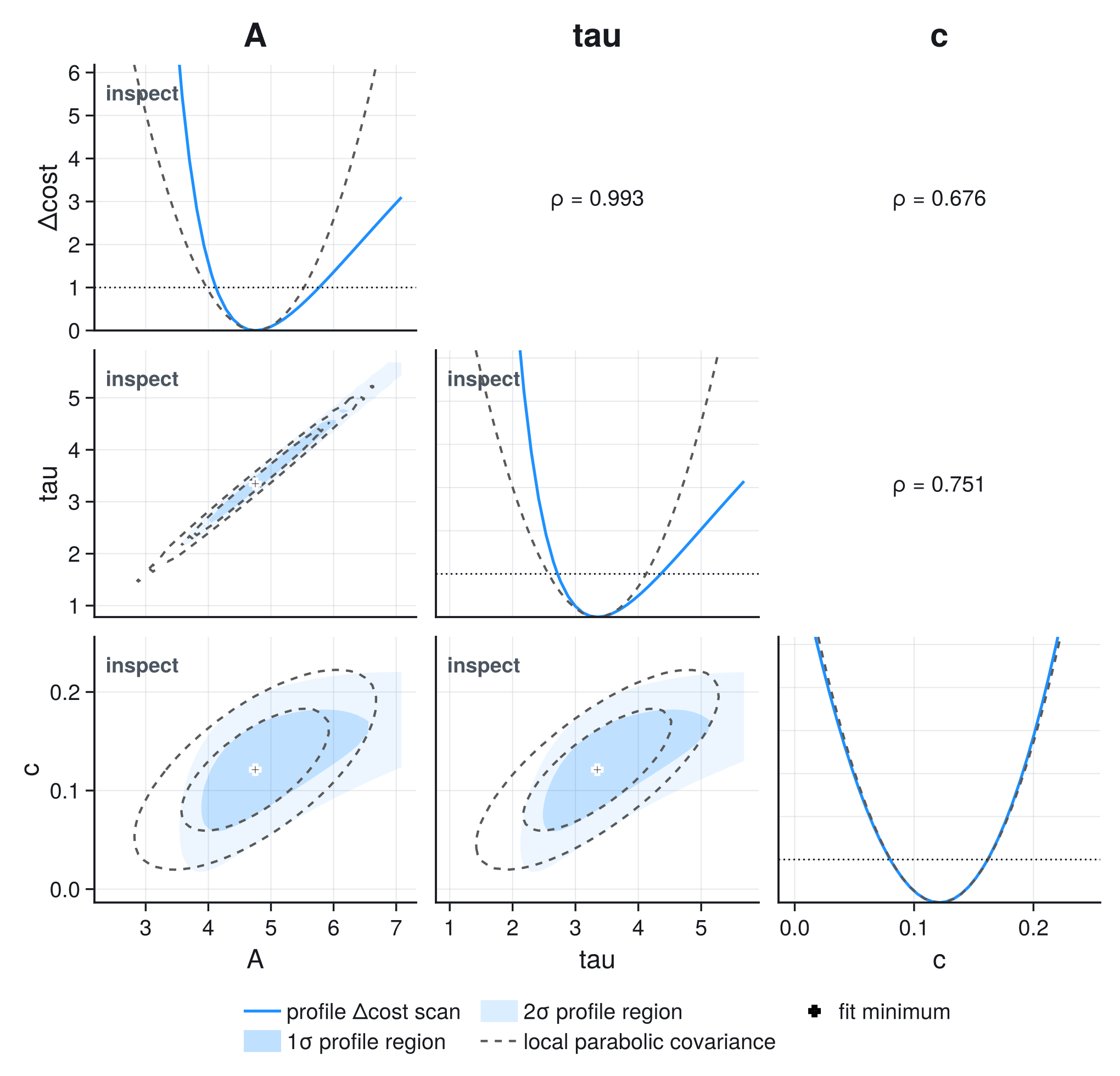
Diagonal: refitted one-parameter profiles against the local parabolic approximation. Lower triangle: filled one- and two-sigma profiled regions against dashed local covariance ellipses. Upper triangle: local correlation coefficients.
Read the diagonal for skewed crossings (asymmetric errors), the lower triangle for bending or displaced region boundaries (the local ellipse is inadequate), and the upper-triangle correlation as a pointer to pairs worth checking.
interval = profile_interval(result, 1; threshold=1.0)
# Qualified because Makie also exports `contour`.
pair = ScientificFitting.contour(result, 1, 2; levels=[2.30, 6.18], adaptive=true)
matrix = profile_matrix(result; parameters=[1, 2, 3], adaptive=true)

profile_findings = diagnose(interval.profile_result)
pair_findings = diagnose(pair; local_covariance=result.param_covariance[[1, 2], [1, 2]])
panels_to_review = filter(p -> last(p) != :ok, matrix.panel_status)
The scans are Makie-free; load CairoMakie only to render them. The Constraints and Profiles example shows the complete workflow.
Observation Likelihoods
Counts, histogram bins, and individual events carry their own sampling process. Writing $p$ for the parameter vector $\theta$, matching the callback argument in the code, the cost for independent observations with normalized density or mass $q_i(y_i\mid f(x_i,p),p)$ is
\[C(p)=-2\sum_i\log q_i(y_i\mid f(x_i,p),p).\]
fit_likelihood_model takes the log probabilities as one vectorized callback; dependent observations need a joint likelihood via fit_custom.
Laplace errors of known scale $b$ have $q(y\mid\mu)=\exp(-|y-\mu|/b)/(2b)$, so $C(\mu)=2\sum_i|y_i-\mu|/b+2n\log(2b)$: the optimum is a sample median, and the cost has corners rather than quadratic curvature:
using ScientificFitting

y = [-1.2, -0.1, 0.2, 0.4, 0.8, 1.3, 5.0]
location(x, p) = fill(p[1], length(x))
# Known scale b = 1; retain the normalizing constant.
logprob(y, mu, p) = -abs.(y .- mu) .- log(2.0)
result = fit_likelihood_model(location, collect(eachindex(y)), y;
    logprob, p0=[0.1], solver=:nelder_mead)
(location=round(only(result.params); digits=6), local_error=only(result.param_stderr))
(location = 0.4, local_error = NaN)Nelder-Mead does not differentiate this cost; its default parameter_covariance=:none leaves the local error unavailable rather than fabricated. Profiles still evaluate the actual cost over explicit values.
A Moving Support Boundary
For a trigger time $\mu$ followed by exponential delays of known scale $b$ ($Y_i=\mu+E_i$, density $q(y\mid\mu)=e^{-(y-\mu)/b}/b$ for $y\ge\mu$), the likelihood is zero for $\mu>\min_i y_i$ and within its support
\[\hat\mu=\min_i y_i,\qquad \Delta C(\mu)=\frac{2n}{b}(\hat\mu-\mu),\quad\mu\le\hat\mu.\]
There is no parabolic minimum, and since $\hat\mu-\mu=\min_i E_i$ with $P(\min_i E_i>t)=P(E_1>t)^n=e^{-nt/b}$, the gap $\hat\mu-\mu$ is exponential with rate $n/b$: the interval $[\hat\mu-db/(2n),\hat\mu]$ covers with probability $1-e^{-d/2}$, so the usual $d=1$ threshold covers only 39.3%. For 68.3% use $d=-2\log(1-0.683)$. This is a property of the sampling model; non-regular likelihoods need their own calibration.
Poisson Counts And Histograms
For an observed count $n_i$ with expectation $\mu_i(\theta)>0$,
\[P(n_i\mid\mu_i) = e^{-\mu_i}\frac{\mu_i^{n_i}}{n_i!}, \qquad C(\theta) = 2\sum_i \left[ \mu_i(\theta)-n_i\log\mu_i(\theta)+\log\Gamma(n_i+1) \right].\]
The factorial term is constant for optimization but keeps likelihood values and information criteria on a defined scale. A zero-count bin is not a zero-uncertainty measurement: with $n=0$ and $\mu=0.5$ it contributes a finite cost and a deviance of $1$, where the Gaussian shortcut $\sigma=\sqrt n$ breaks down. For histogram fits with bin edges $e_1 < e_2 < \dots$ and expected total event count $N$ (the total_count keyword of fit_histogram_density, default sum(counts)), integrate the density over each bin,
\[\mu_i(\theta) = N\int_{e_i}^{e_{i+1}} f(x\mid\theta)\,dx\]
(fit_histogram_density integrates; fit_histogram_model takes expected counts directly). The likelihood-ratio statistic against the saturated model is the Poisson deviance
\[D(\theta) = 2\sum_i \left[ \mu_i-n_i+n_i\log\frac{n_i}{\mu_i} \right],\]
with the logarithm term zero for $n_i=0$; it fills the chi-square fields for count fits. Its chi-square calibration is asymptotic and degrades with many very small expected counts.
Unbinned And Extended Likelihoods
For independent observations from a normalized density $f(x\mid\theta)$,
\[C(\theta) = -2\sum_{i=1}^{n}\log f(x_i\mid\theta).\]
If the expected event count carries information, use a Poisson point process with intensity $\lambda(x\mid\theta)$ and integrated rate $\Lambda(\theta)=\int_\Omega \lambda\,dx$:
\[C_\mathrm{ext}(\theta) = 2\Lambda(\theta) -2\sum_{i=1}^{n}\log\lambda(x_i\mid\theta).\]
The constant $2\log n!$ of the Poisson factor is omitted; $n$ is fixed by the data, so comparisons among extended fits of the same events are unaffected, but do not compare this value against a binned Poisson cost, which retains its factorial terms.
fit_unbinned_model uses the density; fit_extended_unbinned_model integrates the intensity over the declared domain. Acceptance, truncation, resolution, and selection must appear in $f$ or $\lambda$.
An unbinned likelihood value is not a goodness-of-fit statistic — its absolute scale depends on density and units — so chi-square fields are NaN for generic unbinned fits. Use an empirical-CDF test, probability-integral transforms, simulation, or a likelihood ratio against a specified alternative.
Model Comparison With AIC And BIC
For $k$ fitted parameters and maximized normalized likelihood $L_{\max}$,
\[\mathrm{AIC}=2k-2\log L_{\max}, \qquad \mathrm{BIC}=k\log n-2\log L_{\max}.\]
Smaller is preferred within a valid comparison. Without observation uncertainties, the profiled $\hat\sigma$ counts toward $k$ (see Unknown Residual Scale). $n$ is the number of observations plus one dimension per Gaussian auxiliary term; likelihood fits take the observation count from the nobs keyword and add the auxiliary dimensions themselves. For strongly correlated data there may be no unique effective sample size, so state what $n$ means before using BIC as evidence. Compare only candidates that share the observations, the likelihood normalization, the treatment of auxiliary information, and the definitions of $n$ and $k$. When Gaussian terms are read as priors, ordinary AIC/BIC lose their maximum-likelihood interpretation. A lower criterion prefers one candidate relative to the others considered — no more.
Reporting Checklist
A reproducible result states:
- observations, units, and selection or binning rules;
- the model and the physical meaning of every parameter;
- the uncertainty or likelihood model, including correlations and auxiliary information;
- the minimized cost, free-parameter count, and goodness-of-fit statistic where its reference distribution is justified;
- whether covariance errors or profile intervals were reported, and the covariance-scaling policy;
- residual, pull, profile, or simulation checks relevant to the model;
- active bounds, fixed parameters, failed scans, or approximations limiting interpretation.
Further Reading
- Particle Data Group: Statistics review — likelihood, goodness of fit, confidence intervals, nuisance parameters, asymptotics.
- Baker and Cousins — chi-square and likelihood functions for histogram fits.
- Wilks — the theorem behind the profile thresholds.
- Akaike — the information criterion.
- York — the classical effective-variance line fit this package generalizes.