Multi-Dataset Fit: Which Parameters May Be Shared?
A simultaneous fit can use shared structure across datasets, but sharing a parameter is a scientific hypothesis, not a numerical convenience.
This controlled calibration-transfer example asks whether three readout channels may use one common gain. The answer is no: channels A and B are compatible, while channel C requires a separate gain.
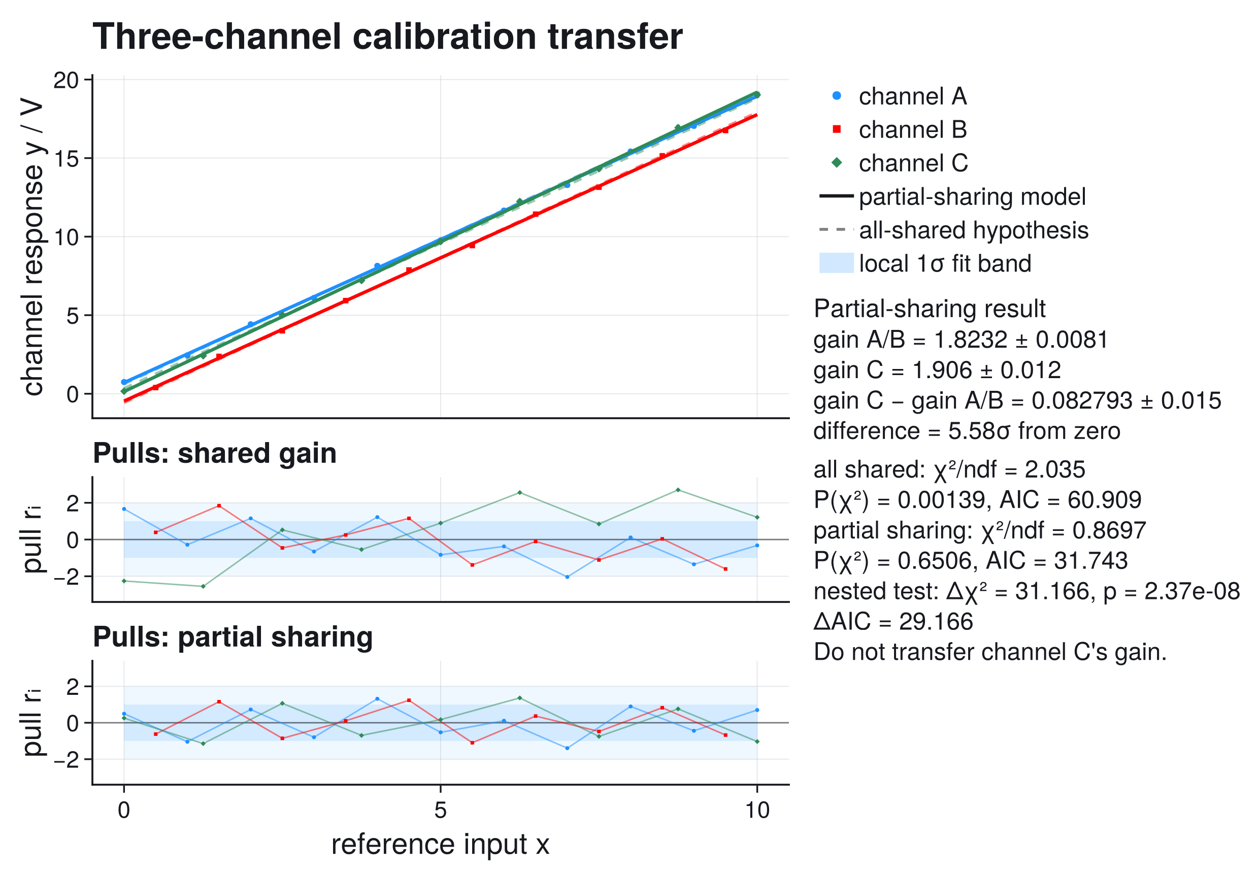
The solid lines show the accepted partial-sharing model; the dashed lines force all channels to one shared gain. In the main panel the difference is easy to underestimate; the first pull panel — residuals in units of their stated uncertainties, defined below — makes the failure of the all-shared hypothesis clear.
The Scientific Question
Three nominally identical readout channels are calibrated against the same reference input. Their electronic zero points may differ, but the proposed transfer procedure assumes one common sensitivity:
\[y_i(x)=g x+b_i, \qquad i\in\{A,B,C\}.\]
If this assumption is valid, one accurately calibrated gain can be transferred between channels after correcting their offsets; if one channel has a different gain, the transfer introduces a systematic error that grows with input.
The teaching record is not attributed to a particular instrument. The three explicit data tables have different x sampling, point-dependent absolute y uncertainties, independent offsets, realistic random scatter, and an incompatible gain in channel C; the fit must recover that incompatibility without using it as an input.
A mental model: the channels share a sensor type but not necessarily the whole electronics chain:
\[\begin{array}{c|c|c} \text{channel} & \text{gain source} & \text{offset source} \\ \hline A & \text{amplifier family 1} & \text{own zero point} \\ B & \text{amplifier family 1} & \text{own zero point} \\ C & \text{replacement amplifier} & \text{own zero point} \end{array}\]
Data
The code below uses three explicit calibration channels. Each channel has its own x grid and point-by-point absolute y uncertainty; the arrays are the complete fit input. The record is constructed for this example rather than measured on an instrument: channel C is built with a deliberately different gain, and the fit must recover that difference without being told. The reference input $x$ and the channel response $y$ are both in volts, so the gains are dimensionless and the offsets are in volts.
The Multi-Dataset Cost
For independent Gaussian measurements, the simultaneous cost is
\[\chi^2(p) = \sum_i \sum_j \left[ \frac{y_{ij}-f_i(x_{ij};p_i)}{\sigma_{ij}} \right]^2.\]
The bracketed quantity is the pull of point $j$ in dataset $i$: its residual $y_{ij}-f_i(x_{ij};p_i)$ divided by its stated uncertainty $\sigma_{ij}$. Under a correct model with correct uncertainties the pulls scatter around zero with width near one; the pull panels display them against $\pm1$ and $\pm2$ reference bands (Residuals And Pulls).
Each local model receives only the global parameters listed by its parameter_map. The first hypothesis uses
\[p_\mathrm{all}=(g,b_A,b_B,b_C),\]
with maps
\[p_A=(p_1,p_2),\qquad p_B=(p_1,p_3),\qquad p_C=(p_1,p_4).\]
All three channels use the same gain $g$.
The second hypothesis uses
\[p_\mathrm{partial}=(g_{AB},b_A,b_B,g_C,b_C),\]
with maps
\[p_A=(p_1,p_2),\qquad p_B=(p_1,p_3),\qquad p_C=(p_4,p_5).\]
Channels A and B share $g_{AB}$; channel C has its own $g_C$.
Complete Fit Code
using Distributions
using ScientificFitting
using LinearAlgebra
using Printf

linear_channel(x, p) = @. p[1] * x + p[2]

x_a = [0.0, 1.0, 2.0, 3.0, 4.0, 5.0, 6.0, 7.0, 8.0, 9.0, 10.0]
y_a = [
    0.744750, 2.444135, 4.420060, 6.098325, 8.141240, 9.763075,
    11.660295, 13.287080, 15.417610, 17.051490, 19.047875,
]
sigma_a = [
    0.075, 0.083, 0.091, 0.099, 0.107, 0.115,
    0.123, 0.131, 0.139, 0.147, 0.155,
]

x_b = [0.5, 1.5, 2.5, 3.5, 4.5, 5.5, 6.5, 7.5, 8.5, 9.5]
y_b = [
    0.391920, 2.378570, 4.007500, 5.927490, 7.877840,
    9.433180, 11.431380, 13.147100, 15.144640, 16.759710,
]
sigma_b = [0.088, 0.094, 0.100, 0.106, 0.112, 0.118, 0.124, 0.130, 0.136, 0.142]

x_c = [0.0, 1.25, 2.5, 3.75, 5.0, 6.25, 7.5, 8.75, 10.0]
y_c = [
    0.159600, 2.417162, 5.013387, 7.207425, 9.690625,
    12.237350, 14.323312, 16.937275, 19.023650,
]
sigma_c = [0.08000, 0.09125, 0.10250, 0.11375, 0.12500,
           0.13625, 0.14750, 0.15875, 0.17000]

models = [linear_channel, linear_channel, linear_channel]
x_sets = [x_a, x_b, x_c]
y_sets = [y_a, y_b, y_c]
sigma_sets = [sigma_a, sigma_b, sigma_c]

all_shared_result = fit_multi_model(
    models,
    x_sets,
    y_sets;
    p0=[1.85, 0.7, -0.4, 0.1],
    sigma_y=sigma_sets,
    parameter_map=[[1, 2], [1, 3], [1, 4]],
    parameter_names=["shared gain", "offset A", "offset B", "offset C"],
)

partial_shared_result = fit_multi_model(
    models,
    x_sets,
    y_sets;
    p0=[1.82, 0.7, -0.4, 1.90, 0.1],
    sigma_y=sigma_sets,
    parameter_map=[[1, 2], [1, 3], [4, 5]],
    parameter_names=["gain A/B", "offset A", "offset B", "gain C", "offset C"],
)

gain_gap_gradient = [-1.0, 0.0, 0.0, 1.0, 0.0]
gain_gap = partial_shared_result.params[4] - partial_shared_result.params[1]
sigma_gain_gap = sqrt(dot(
    gain_gap_gradient,
    partial_shared_result.param_covariance * gain_gap_gradient,
))
delta_chi2 = all_shared_result.stats.chi2 - partial_shared_result.stats.chi2
nested_pvalue = ccdf(Chisq(1), delta_chi2)

println("All-shared-gain hypothesis")
println(report_text(all_shared_result))
println()
println("Partial-sharing model")
println(report_text(partial_shared_result))
@printf("gain C - gain A/B = %.5f +/- %.5f\n", gain_gap, sigma_gain_gap)
@printf("nested test: delta chi2 = %.5f for 1 dof, p = %.4g\n",
        delta_chi2, nested_pvalue)
println()
println("All-shared diagnostic dashboard")
println(diagnostic_dashboard_text(all_shared_result))
println("Partial-sharing diagnostic dashboard")
println(diagnostic_dashboard_text(partial_shared_result))All-shared-gain hypothesis Fit report backend = optimization converged = true iterations = 4 message = Success Parameters: shared gain = 1.8478 +/- 0.0068 offset A = 0.620 +/- 0.040 offset B = -0.566 +/- 0.045 offset C = 0.340 +/- 0.045 Statistics: cost = multi_chi2 cost_min = 52.9085 minus2loglik_min = 52.9085 chi2 = 52.9085 ndf = 26 chi2/ndf = 2.03494 pvalue = 0.00139032 AIC = 60.9085 BIC = 66.5133 Partial-sharing model Fit report backend = optimization converged = true iterations = 5 message = Success Parameters: gain A/B = 1.8232 +/- 0.0081 offset A = 0.707 +/- 0.043 offset B = -0.465 +/- 0.048 gain C = 1.906 +/- 0.012 offset C = 0.139 +/- 0.057 Statistics: cost = multi_chi2 cost_min = 21.7427 minus2loglik_min = 21.7427 chi2 = 21.7427 ndf = 25 chi2/ndf = 0.869707 pvalue = 0.650557 AIC = 31.7427 BIC = 38.7487 gain C - gain A/B = 0.08279 +/- 0.01483 nested test: delta chi2 = 31.16586 for 1 dof, p = 2.369e-08 All-shared diagnostic dashboard Fit diagnostic dashboard status = review - inspect diagnostics critical = 0, warning = 1, info = 0 1 warning(s). Inspect before trusting uncertainties or conclusions. Next actions: 1. Treat the result as suspicious unless you can explain the residual pattern or uncertainty model. Partial-sharing diagnostic dashboard Fit diagnostic dashboard status = ok - no immediate issue critical = 0, warning = 0, info = 0 No major diagnostic issues detected by the current checks. No next action required by the current diagnostic checks.
The automatic dashboard marks the all-shared fit for review from its large reduced chi-square and small p-value. Those aggregate checks establish that the stated model and uncertainties are inconsistent with the data but cannot identify which sharing assumption failed; the per-dataset pulls localize it, and the nested test and propagated gain difference quantify the evidence for freeing channel C's gain.
Diagnose The All-Shared Hypothesis
The fully shared model converges; its fitted gain is a compromise between incompatible channels:
\[g_\mathrm{all}=1.8478\pm0.0068.\]
The fit gives
\[\frac{\chi^2_\mathrm{all}}{\mathrm{ndf}}=2.035, \qquad P(\chi^2_\mathrm{all})=0.00139.\]
Here ndf counts all points across datasets minus the global free parameters: $11+10+9-4=26$ for the all-shared model and $30-5=25$ for partial sharing (Degrees Of Freedom).
The first pull panel shows the specific failure: channel C is systematically below the common-gain model at low input and above it at high input — the residual signature of a slope mismatch. Channels A and B are pulled in the opposite direction because the shared gain must compromise.
Fit Only The Defensible Sharing Structure
Allowing channel C to have an independent gain gives
\[g_{AB}=1.8232\pm0.0081, \qquad g_C=1.9060\pm0.0124.\]
The gain difference must be propagated from the joint covariance matrix:
\[\Delta g = g_C-g_{AB}, \qquad \sigma_{\Delta g}^2 = \nabla\Delta g^\mathsf{T} \operatorname{Cov}(p) \nabla\Delta g.\]
Here,
\[\Delta g=0.0828\pm0.0148,\]
which differs from zero by approximately $5.6\sigma$ under the local Gaussian approximation.
The revised fit gives
\[\frac{\chi^2_\mathrm{partial}}{\mathrm{ndf}}=0.870, \qquad P(\chi^2_\mathrm{partial})=0.651.\]
The second pull panel no longer contains a channel-dependent trend. Sharing the gain between A and B is supported by this dataset; transferring channel C's gain is not.
Decision: Test The Nested Sharing Hypothesis
The partial-sharing model is obtained from the all-shared model by freeing one parameter: $g_C$ no longer has to equal $g_{AB}$. Under the independent Gaussian model with known standard deviations, the cost difference
\[\Delta\chi^2 = \chi^2_\mathrm{all}-\chi^2_\mathrm{partial} = 31.166\]
is compared with a chi-square distribution with one degree of freedom. The result is
\[P\!\left(\chi^2_1 \geq 31.166\right) = 2.37\times10^{-8}.\]
This is the direct test of the equality constraint $g_C=g_{AB}$; it agrees with the approximately $5.6\sigma$ gain difference from the joint covariance, as expected for a linear Gaussian problem, where $\Delta\chi^2=(\Delta g/\sigma_{\Delta g})^2$: $\sqrt{31.166}=5.58$, matching the $5.6\sigma$ above. In a nonlinear or bounded problem, profile the difference instead of assuming a symmetric Gaussian error.
AIC As A Cross-Check
A lower $\chi^2$ is expected from one extra parameter even if the freedom is unnecessary; AIC adds a parameter-count penalty:
\[\mathrm{AIC}=2k-2\log L_{\max},\]
where $k$ is the number of free parameters and $L_{\max}$ the maximized likelihood. fit_multi_model minimizes the summed chi-square without the constant Gaussian normalization terms $\sum_{ij}\log(2\pi\sigma_{ij}^2)$, so the printed values are $\mathrm{AIC}=\chi^2_{\min}+2k$ — for the all-shared model $52.9085 + 2\cdot 4 = 60.9085$. The dropped constant is the same for both models (same data, same $\sigma_{ij}$), so only the difference is meaningful (Model Comparison With AIC And BIC):
\[\Delta\mathrm{AIC} = \mathrm{AIC}_\mathrm{all}-\mathrm{AIC}_\mathrm{partial} = 60.9085-31.7427 = 29.17 = \Delta\chi^2-2.\]
The improvement is far larger than the $+2$ penalty for the one extra gain parameter. AIC only compares the candidate models supplied here: a nonlinear response, correlated calibration errors, or a shared reference-standard uncertainty could still require another model.
What The Bands Mean
The main panel shows one local 1σ fit band for each channel under the partial-sharing model. For a local linear model,
\[\sigma_\mathrm{fit}^2(x) = J(x)\,\operatorname{Cov}(p_i)\,J^\mathsf{T}(x), \qquad J(x)=(x,1),\]
where $\operatorname{Cov}(p_i)$ is the $2\times2$ block of the joint fit covariance belonging to channel $i$'s (gain, offset) pair; it carries the gain–offset correlation, and the A and B bands are correlated through the shared gain.
These bands describe uncertainty in each fitted mean response; they are not prediction bands for a future observation and do not add $\sigma_{ij}^2$, uncertainty in the reference x values, or correlations caused by a shared calibration standard.
What Can Go Wrong
- Sharing by naming convention: parameters should be shared because the physical model requires it, not because two columns have the same label.
- Reading only the aggregate fit statistic: one failing dataset can be hidden inside an acceptable-looking global curve.
- Fitting every dataset independently: this discards real shared information and prevents direct propagation through the joint covariance.
- Ignoring shared systematic uncertainty:
fit_multi_modelcurrently supports dataset-specific diagonalsigma_y; a common reference-standard error requires a richer covariance treatment than this example.
Reproduce The Figure
The tracked script contains the complete fits, covariance propagation, pull construction, local bands, and light/dark Makie figure:
julia --project=docs examples/gallery/10_multi_dataset_calibration.jlTransfer the gain between channels A and B; calibrate channel C separately.
Next, use Full Covariance when datasets share systematic uncertainty, or Constraints and Profiles when the shared-parameter geometry is nonlinear and local errors may fail.