ScientificFitting.jl

Nonlinear curve and likelihood fitting with explicit uncertainties: y errors, x errors, full covariance matrices, matrix-free whitening, Poisson and unbinned likelihoods, parameter priors and constraints, profile-likelihood intervals, diagnostics, and Makie figures — one workflow from data to reported result, in Julia and from Python.

using ScientificFitting

x = [0.5, 1.0, 1.5, 2.0, 2.5, 3.0, 3.5, 4.0]
U = [1.31, 2.13, 3.09, 3.90, 5.15, 5.95, 7.11, 7.86]
sigma_U = fill(0.12, length(U))

result = fit_model((x, p) -> p[1] .* x .+ p[2], x, U;
                   p0=[1.0, 0.0], sigma_y=sigma_U)
println(report_text(result; parameter_names=["m", "b"]))

Fit report
backend = lsqfit
converged = true
iterations = unavailable
message = Converged with LsqFit

Parameters:
  m = 1.919 +/- 0.037
  b = 0.246 +/- 0.094

Statistics:
  cost = chi2
  cost_min = 6.03671
  minus2loglik_min = -13.1845
  chi2 = 6.03671
  ndf = 6
  chi2/ndf = 1.00612
  pvalue = 0.419091
  AIC = -9.18449
  BIC = -9.02561

One call renders the same kind of fit as a publication-ready figure with a result panel (fitplot, from the Quickstart):

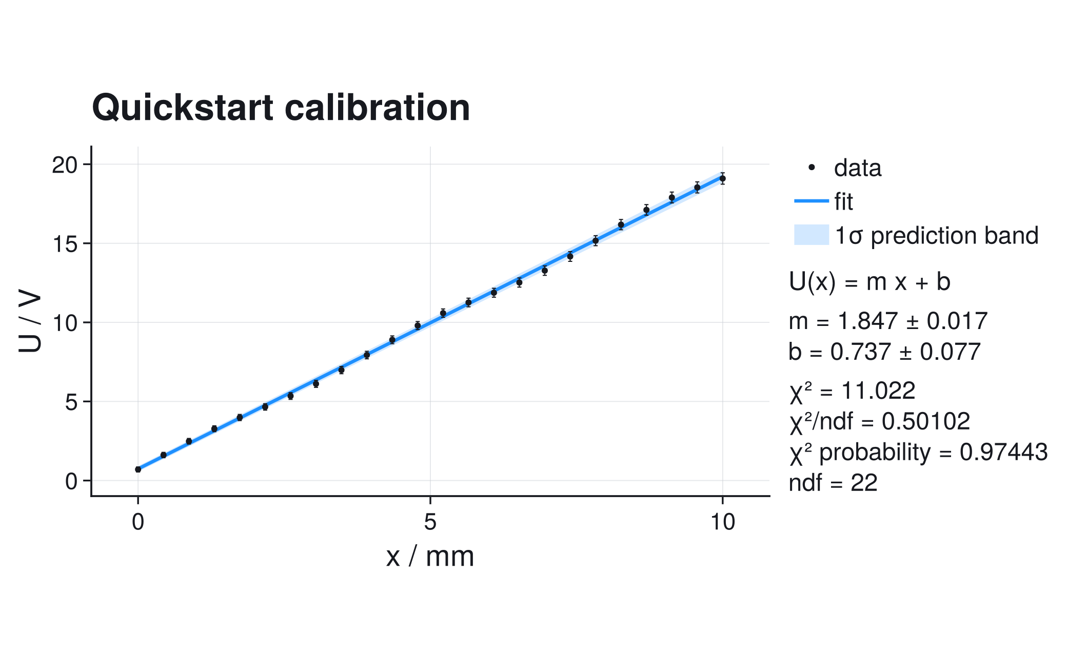
Linear calibration fit with data, fitted line, prediction band, and result panel

Where to go next:

First complete fit, including the plot and the diagnosis: Quickstart.
Which function fits your data: the entry-point table.
Complete executable analyses, from x-y uncertainties to an LHCb mass spectrum: Gallery.
What the numbers mean, derived once and precisely: Statistics Reference.
What this package does not do: Scope and Alternatives.