Packages And Interfaces
Fit distribution objects, attach named parameters, and select a solver. The LHCb mass spectrum combines these interfaces on collision data.
The distribution-object, BuildConstructors and NativeMinuit adapters below require ScientificFitting 0.3 or later plus their optional packages. The Python API uses NumPy callbacks and Matplotlib; it does not wrap these Julia-specific objects.
Probability Models
| Package | Interface in ScientificFitting |
|---|---|
| Distributions.jl | Pass a function p -> distribution to fit_distribution to model the observations themselves, or a fixed distribution as the error keyword of fit_likelihood_model to model additive residuals. Supports continuous, discrete and multivariate observations. |
| NumericalDistributions.jl | Numerically normalized densities, also inside mixtures and products. Bin probabilities use a CDF or adaptive quadrature when no CDF is available. |
| DistributionsHEP.jl | Reuse compatible shapes and native ExtendedMixtureModel objects. Extended fits retain component yields for both event samples and histograms. |
Supply a function that constructs the distribution from parameter vector p; five illustrative observations determine a Gaussian center and scale:
using ScientificFitting, Distributions, OptimizationOptimJL

observations = [4.8, 5.1, 5.6, 5.4, 5.0]
normal_model(p) = Normal(p[1], exp(p[2]))  # p[2] = log(scale), so scale > 0
result = fit_distribution(normal_model, observations; p0=[5.0, log(0.4)])
println(report_text(result))
Fit report
backend = optimization
converged = true
iterations = 7
message = Success
Parameters:
p1 = 5.18 +/- 0.13
p2 = -1.25 +/- 0.32
Statistics:
cost = distribution_likelihood
cost_min = 1.65976
minus2loglik_min = 1.65976
chi2 = NaN
ndf = 3
chi2/ndf = NaN
pvalue = NaN
AIC = 5.65976
BIC = 4.87863
Diagnosis:
[WARNING] Goodness-of-fit statistic is unavailable
evidence: The fit does not provide a finite chi-square-like goodness-of-fit statistic.
action: Use residual diagnostics, profiles, simulation, or a likelihood-specific goodness-of-fit test instead of interpreting p-values.fit_distribution models the observations themselves. A fixed error distribution instead describes additive noise around predictions:
x, y = [0., 1., 2., 3.], [0.1, 1.2, 1.8, 3.4]
line(x, p) = @. p[1]*x + p[2]
regression = fit_likelihood_model(line, x, y;
    error=Normal(0, 0.2), p0=[1., 0.])
println("Slope, intercept: ", round.(regression.params; digits=4))
Slope, intercept: [1.05, 0.05]For multivariate samples pass a matrix and set obsdim=1 (events in rows) or obsdim=2 (events in columns); each vector observation uses its joint density (dependence needs a joint likelihood).
Automatic differentiation passes dual numbers through the model-construction function, so do not force Float64 inside it (for example via Float64(p[1]) or a Vector{Float64} buffer); if that is unavoidable, select derivatives=:finite. See Distribution Objects for support, truncation and bin-boundary conventions.
Named Model Construction
BuildConstructors.jl attaches names, starts, bounds and fixed values to model parameters. Reusing a name shares that parameter between components.
Data: illustrative counts in 20 equal bins on $[0,10]$. Model: a Gaussian peak with fixed width $0.4$, plus a uniform background. Fit the center and expected signal/background counts $N_s,N_b$. Both densities are normalized within the observation window. With bin edges $e_1<\dots<e_{21}$ and normalized signal and background densities $f_s$ and $f_b$, the expected count in bin $i$ is
\[\mu_i=N_s\int_{e_i}^{e_{i+1}}f_s(x)\,dx +N_b\int_{e_i}^{e_{i+1}}f_b(x)\,dx.\]
The uniform component contributes $N_b/20$ to each bin; the fit uses these integrals as Poisson means.
using BuildConstructors, DistributionsHEP

@with_parameters(Peak; center::P, width::P, window::Tuple{Float64,Float64}, begin
    truncated(Normal(center, width), window...)
end)

@with_parameters(Spectrum; peak, background, signal_yield::P, background_yield::P, begin
    ExtendedMixtureModel(
        [build_model(peak, pars), background],  # build the nested component
        [signal_yield, background_yield],
    )
end)

constructor = ConstructorOfSpectrum(
    ConstructorOfPeak(
        AdvancedParameter("center", 5.0; boundaries=(4.0, 6.0)),
        AdvancedParameter("width", 0.4; fixed=true), (0.0, 10.0)),
    Uniform(0.0, 10.0),
    AdvancedParameter("signal_yield", 70.0; boundaries=(0.0, 200.0)),
    AdvancedParameter("background_yield", 40.0; boundaries=(0.0, 200.0)),
)
edges = collect(0.0:0.5:10.0)
counts = [2, 1, 3, 1, 2, 2, 1, 1, 3, 14, 33, 22, 7, 2, 1, 2, 3, 1, 1, 2]

optim = fit_distribution(constructor, edges, counts;
    solver=OptimizationSolver(LBFGS()), tol=1e-7)
println(report_text(optim))
Fit report
backend = optimization
converged = true
iterations = 4
message = Success
Parameters:
center = 5.364 +/- 0.059
width = 0.4 +/- 0.0 (fixed)
signal_yield = 70.1 +/- 9.0
background_yield = 33.9 +/- 6.6
Statistics:
cost = histogram_poisson_likelihood
cost_min = 62.0509
minus2loglik_min = 62.0509
chi2 = 4.82081
ndf = 17
chi2/ndf = 0.283577
pvalue = 0.998233
AIC = 68.0509
BIC = 71.0381::P marks a parameter descriptor; plain fields such as window and background are fixed structural arguments, filled positionally (here (0.0, 10.0) and Uniform(0.0, 10.0)). Conflicting metadata for shared names is rejected. Inside the begin ... end body, the macro supplies pars, the container of current parameter values (the second argument of the generated build_model method); pass it through to nested constructors — build_model(peak, pars) resolves the peak's parameters from the same container — while a plain distribution such as background is used as-is. fixed=true treats the width as exactly known; an uncertain calibration needs an explicit parameter constraint, not uncertainty metadata.
A normalized distribution needs the keyword total_count (the known expected event count on its full support); an ExtendedMixtureModel carries its component yields, so omit it here. For individual events use fit_distribution(constructor, events; solver=...).
Minimizers
| Package | Role and current integration |
|---|---|
| LsqFit.jl | Levenberg-Marquardt for compatible Gaussian residual problems; used by the least-squares path. |
| Optimization.jl / Optim.jl | Solver interface / Julia algorithms for scalar objectives. Select OptimizationSolver(algorithm); bounds and nonlinear constraints require a compatible algorithm. |
| NativeMinuit.jl | Optional Julia-native adapter for MIGRAD, Minuit's gradient-based minimizer: NativeMinuitSolver(). Requires Julia 1.11+ for NativeMinuit 0.7; the core still supports Julia 1.10. |
| NLopt.jl | Provides the bounded Nelder-Mead path, solver=:nelder_mead. Derivative-free fitting is typically chosen for non-smooth costs, so parameter_covariance=:auto selects :none on this path: free-parameter errors are NaN; supply explicit profile ranges instead. |
| NonlinearSolve.jl | Julia residual-based solvers; not currently integrated. |
| Minuit2.jl | Julia bindings to C++ Minuit2; distinct from NativeMinuit and not currently integrated. |
Change the solver without rebuilding the statistical model:
import NativeMinuit  # load the extension without importing NativeMinuit.profile

minuit = fit_distribution(constructor, edges, counts;
    solver=NativeMinuitSolver(), tol=1e-3)

for (label, fit) in (("Optim", optim), ("MIGRAD", minuit))
    println(label, ": center = ", round(parameter_values(fit).center; digits=5),
        "; -2 log L = ", round(fit.stats.cost_min; digits=5))
end
Optim: center = 5.3644; -2 log L = 62.05092
MIGRAD: center = 5.3644; -2 log L = 62.05092Julia's import avoids the profile name clash.
Omit tol for solver defaults: 1e-10 for Optim with automatic derivatives, 1e-6 with finite differences, and MIGRAD's native 0.1. This example sets both tolerances explicitly — 1e-7 for Optim and 1e-3 in place of MIGRAD's native 0.1 — so both costs agree within 1e-6.
The adapter sets errordef=1, Minuit's convention that a cost increase of 1 marks one standard error, matching the $-2\log L$ scale; the covariance policy and the native result.solver_result.raw object are specified in Solver Adapters.
Reuse Results And Profile Scans
model = fitted_model(minuit)  # returns DistributionsHEP.ExtendedMixtureModel
values = parameter_values(minuit)  # named values, including fixed parameters
println("Center: ", round(values.center; digits=4))
println("Expected count: ", round(DistributionsHEP.total_yield(model); digits=3))

# Re-optimize the yields at each trial center; retain the chosen solver.
scan = profile(minuit, 1; nsigma=2.5, npoints=25, on_failure=:throw)
interval = profile_interval(scan)
println("Profile interval: ", round(interval.lower; digits=3),
    " to ", round(interval.upper; digits=3))
Center: 5.3644
Expected count: 103.995
Profile interval: 5.306 to 5.423model(x) evaluates the fitted intensity (expected events per unit $x$, the density times the total yield); MixtureModel(model) gives the normalized distribution. Reconstruction and plotting do not refit.
Coverage and failure modes of the $\Delta(-2\log L)=1$ crossing are derived in Profiles and Contours; increase the grid resolution before quoting more digits.
local_sigma overlays the parabola implied by the local standard error, $\Delta=((\theta-\hat\theta)/\sigma)^2$; agreement with the profile curve indicates a nearly quadratic cost.
using CairoMakie  # only needed for the figure
plot_options = (local_sigma=minuit.param_stderr[1],
    title="Component-location likelihood", xlabel="center",
    ylabel="Delta (-2 log L)")
fig = plot_profile(scan; plot_options...)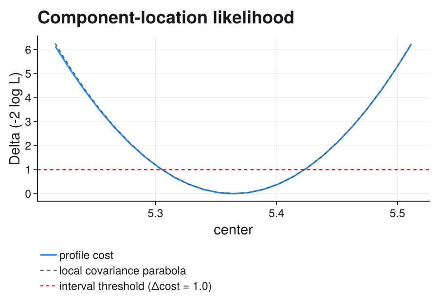
Posterior Inference
Turing's external-likelihood interface reuses a ScientificFitting (SF) data likelihood directly; no extension is needed. Here eight illustrative counts, taken under identical conditions (equal exposure), share one rate $r$: $n_i\sim\operatorname{Poisson}(r)$. The prior $r\sim\operatorname{Gamma}(2,3)$ uses shape and scale. It is conjugate to the Poisson rate: the posterior shape gains the total count, and the posterior rate (the inverse scale, $1/3$ for this prior) gains one unit of exposure per observation, so the exact posterior is $\operatorname{Gamma}(2+\sum_i n_i,\;[1/3+8]^{-1})$.
Install Turing and FlexiChains for this example, tested with Turing 0.48. NUTS, Turing's gradient-based Hamiltonian Monte Carlo sampler (here 500 adaptation steps, target acceptance 0.85, and four serial chains of 2000 draws), requires a differentiable log likelihood in the chosen parameterization.
using ScientificFitting, Distributions, Turing, Random, Statistics, Printf
using FlexiChains: rhat, ess, Extra

counts = [0, 3, 1, 4, 2, 5, 0, 2]
mle = fit_distribution(p -> Poisson(p[1]), counts;
    p0=[2.], bounds=([0.], [Inf]))
data_cost = mle.problem.objective  # full data -2log(L), constants retained; no SF priors or constraints

@model function rate_posterior(data_cost)
    rate ~ Gamma(2., 3.)  # specify the prior once, here
    @addlogprob! -data_cost([rate])/2
end

posterior = rate_posterior(data_cost)
chain = sample(Xoshiro(20260912), posterior, NUTS(500, .85; adtype=AutoForwardDiff()),
    MCMCSerial(), 2000, 4; progress=false, verbose=false)
draws = chain[@varname(rate)]  # Turing 0.48 returns a FlexiChains chain
exact = Gamma(2 + sum(counts), inv(1/3 + length(counts)))
@printf("Maximum likelihood: %.3f\n", only(mle.params))
@printf("Posterior mean / sd: sampled %.3f / %.3f; exact %.3f / %.3f\n",
    mean(draws), std(draws), mean(exact), std(exact))
@printf("R-hat: %.4f; bulk ESS: %.0f; divergent transitions: %d\n",
    rhat(chain)[@varname(rate)], ess(chain)[@varname(rate)],
    count(chain[Extra(:numerical_error)]))
Maximum likelihood: 2.125
Posterior mean / sd: sampled 2.296 / 0.539; exact 2.280 / 0.523
R-hat: 1.0010; bulk ESS: 2715; divergent transitions: 0The posterior mean differs from the maximum-likelihood estimate because it includes the prior. $\widehat R$ near 1 (below about 1.01) means the four chains agree; the effective sample size (ESS) counts roughly independent draws; any divergent transitions signal unreliable exploration. These diagnose sampling, not whether the Poisson model describes the experiment.
LikelihoodFitResult.problem.objective does not transfer SF bounds, fixed parameters or auxiliary parameter terms; define the corresponding support and auxiliary observations explicitly in Turing. Here the bound $r\ge 0$ needs no extra handling, because Turing samples a Gamma-distributed variable on an internally transformed (log) scale that keeps it positive. Do not reuse a penalized cost as data, count a prior twice, or treat a custom loss as a log likelihood unless it matches the cost convention. Posterior credible intervals are not profile confidence intervals.
Related Workflows
These packages offer different modeling workflows, not interchangeable minimizers:
| Package | When to consider it |
|---|---|
| RooFit / RooFitLite.jl | Compositional probability modeling in ROOT / a RooFit-style Julia interface. ScientificFitting does not convert their model graphs. A custom likelihood callback is possible if you supply a compatible scalar objective; that is not a native adapter. |
| GLM.jl | Linear/generalized linear models with formulas, tables and link functions. |
| Turing.jl | Probabilistic models and posterior inference. Reuse a data likelihood as above; a posterior sampler is not a drop-in minimizer. |
For kafe2's influence and software attribution, see Citation and License.